by Shawn Burke, Ph.D.
SUMMARY
A method for power ranking paddlers based on race finishing time is proposed. The method relies on some basic physics, careful bookkeeping of race results, and an analysis package like Matlab or R that can manipulate matrices and compute pseudo-inverses. Simple examples are presented for solo and tandem paddlers.
INTRODUCTION
For some time, I’ve wondered if you can rank paddlers by their padding power, computed using race timing results. By comparison, the NECKRA (New England Canoe and Kayak Racing Association) Points Series relies on finishing order to score paddlers. I wanted something grounded in physics.
Using finishing times to infer paddling power is complicated by three factors: (1) the nonlinear dependence between hull speed and power; (2) tandem teams and the need to distinguish their individual contributions to hull speed; and (3) multiple race results over the course of a season for each participating paddler. Now a little bit of physics from Part 1: Tandem vs. Solo can address the first concern. And some matrix algebra I have used extensively (singular valued decompositions and related analysis) addresses the other two.
While drinking my morning coffee I realized that the key is to use a Moore-Penrose pseudo-inverse after taking into account the nonlinear dependence of finishing time on power. That about sums it up, so feel free to going back to what you were doing if you wish. If, however, you’d like to learn more pull up a chair, pour a glass of your favorite beverage, and let’s have some fun. What follows is a more mathematical Science of Paddling article than Part 29. Yay!
THE MODEL
We know from Part 1: Tandem vs. Solo, as well as from Part 26: Waking Up, that the cruising speed of a hull v is equal to the cube root of the paddling power in the hull P multiplied by a scaling factor that takes into account the hull’s hydrodynamic characteristics:
![v=\frac{1}{\sqrt[3]{\alpha}} \sqrt[3]{P}](https://s0.wp.com/latex.php?latex=v%3D%5Cfrac%7B1%7D%7B%5Csqrt%5B3%5D%7B%5Calpha%7D%7D+%5Csqrt%5B3%5D%7BP%7D&bg=ffffff&fg=000&s=0&c=20201002)
The scaling factor here is written in an odd way – the inverse of a cube root – in order to make the subsequent analysis a bit cleaner.
From high school physics we know that distance traveled by a hull D is equal to its average speed multiplied by elapsed time T. Expressed in terms of the speed, this means

Equating the speed v in the equations above yields an expression for distance and time in terms of paddling power,
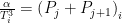
![\frac{D}{T} = \frac{1}{\sqrt[3]{\alpha}} \sqrt[3]{P}](https://s0.wp.com/latex.php?latex=%5Cfrac%7BD%7D%7BT%7D+%3D+%5Cfrac%7B1%7D%7B%5Csqrt%5B3%5D%7B%5Calpha%7D%7D+%5Csqrt%5B3%5D%7BP%7D&bg=ffffff&fg=000&s=0&c=20201002)
In order to determine paddling power P in terms of time T we cube both sides of this equation to yield

See; that’s why the hydrodynamic term 

where 
Consistent with these assumptions, where the finishing times have been appropriately normalized, the paddling power in a given i=th hull is expressed in terms of finishing time and the hull scaling constant

Those of you who are familiar with NECKRA’s Point Series will recognize that the scaling constant
Given multiple race finishing times, appropriately normalized, we can then infer relative paddling power for each paddler. For the moment we’ll assume that the scaling constant
![{\mathbf{y}}_{i} = \left[ \begin{matrix} {T}_{i}^{-3} \\ \vdots \\ {T}_{N}^{-3} \\ \end{matrix} \right]](https://s0.wp.com/latex.php?latex=%7B%5Cmathbf%7By%7D%7D_%7Bi%7D+%3D+%5Cleft%5B+%5Cbegin%7Bmatrix%7D++%7BT%7D_%7Bi%7D%5E%7B-3%7D%C2%A0+%5C%5C++%5Cvdots+%5C%5C++%7BT%7D_%7BN%7D%5E%7B-3%7D%C2%A0+%5C%5C++%5Cend%7Bmatrix%7D+%5Cright%5D&bg=ffffff&fg=000&s=0&c=20201002)
for the N paddlers in that race. So, for M races, the vector of race times is just a stacked collection of yi vectors, vis
![\mathbf{y} = \left[ \begin{matrix} {\mathbf{y}}_{i=1} \\ \vdots \\ {\mathbf{y}}_{i=M} \\ \end{matrix} \right]](https://s0.wp.com/latex.php?latex=%5Cmathbf%7By%7D+%3D+%5Cleft%5B+%5Cbegin%7Bmatrix%7D++%7B%5Cmathbf%7By%7D%7D_%7Bi%3D1%7D%C2%A0+%5C%5C++%5Cvdots+%5C%5C++%7B%5Cmathbf%7By%7D%7D_%7Bi%3DM%7D%C2%A0+%5C%5C++%5Cend%7Bmatrix%7D+%5Cright%5D&bg=ffffff&fg=000&s=0&c=20201002)
Similarly, a vector of paddler powers p can be written as
![\mathbf{p} = \left[ \begin{matrix} {P}_{1} \\ \vdots \\ {P}_{K} \\ \end{matrix} \right]](https://s0.wp.com/latex.php?latex=%5Cmathbf%7Bp%7D+%3D+%5Cleft%5B+%5Cbegin%7Bmatrix%7D++%7BP%7D_%7B1%7D%C2%A0+%5C%5C++%5Cvdots+%5C%5C++%7BP%7D_%7BK%7D%C2%A0+%5C%5C++%5Cend%7Bmatrix%7D+%5Cright%5D&bg=ffffff&fg=000&s=0&c=20201002)
for K paddlers participating in a race series. Consequently,

where the elements of the matrix M are either 1’s or 0’s depending on whether a paddler participates in any given race. Within M rows correspond to races, while columns correspond to paddlers. A matrix entry of 1 “connects” a given paddler with their time results for the race in the corresponding row of the y vector. So, in order to determine the relative power of each paddler across a series of races, one solves for the vector p in terms of the timing results vector y and the “connecting” matrix M. Voila!
Those of you who are familiar with linear algebra will be tempted to solve for p in the equation above by taking the inverse of the matrix M, then multiplying this inverse and the vector y. But then you’ll stop and say, “Wait; that matrix isn’t square! I can’t compute the inverse of a non-square matrix.” Which takes us to the land of pseudo inverses and over-determined systems.
Over the course of a race series the number of participating paddlers will be less than the number of timing results they generate. This is why the matrix M will have more rows (corresponding to race results) than columns (corresponding to the racers). Rather than computing

We instead compute

where M+ is the pseudo-inverse of the matrix M. The pseudo-inverse of our non-square matrix satisfies

In other words, the product of a matrix and its pseudo-inverse MM+ acts like the identity matrix I in that it maps all the columns of M to themselves.[4] The pseudo-inverse lets us solve an over-determined system of coupled linear equations,[5] producing a result that is the least-squares best fit to data.
SOLO RACERS EXAMPLE
In order to make this a bit more concrete, let’s look at a simple example using simulated results from two races. In the first race five (5) solo paddlers participate, while in the second race three (3) of those five solo paddlers participate. In the first race the normalized finishing times are:
Paddler 1: 60 min
Paddler 2: 60.5 min
Paddler 3: 62 min
Paddler 4: 63 min
Paddler 5: 63.5 min
In the second race:
Paddler 2: 60 min
Paddler 5: 61 min
Paddler 3: 63 mi
The vector of normalized inverse cube solo finishing times for these two races is then
There are two ‘1’ values in this vector; each corresponds to the fastest finishing time in the two races, normalized to one hour. The numbers after these are ordered from fastest to slowest in each race. Those values are smaller than 1 because we are taking the inverse of their cube, which will always be less than one since the times of the corresponding paddlers is slower (e.g., larger) than for the winner of each race.
We’ve used the first race to “name” our paddlers Paddler 1, Paddler 2, etc. This means that Paddlers 1 and 4 did not participate in the second race. The matrix M is then
We used the first race to establish a one-to-one correspondence between each racer and their results, ranked by finishing times.[6] This is embodied in the first five rows of the matrix, which of course is the identity matrix; the column locations correspond to the relative finishing positions (but not times) since we rank-ordered the timing vector y. The next three rows in M show that only three of the original five paddlers participated, and their relative finishing positions are reflected in the positions of the non-zero elements of the lower 3-row submatrix. Taking the pseudo-inverse of this matrix and multiplying it by the matrix of normalized inverse cube solo finishing times yields the relative power values for these five paddlers:[7]
Even though Paddler 1 didn’t participate in the second race, they have the highest relative power because they finished higher than Paddler 2 in the first race, by 30 seconds. Paddler 5 rose in the ranks after their 5th pace finish in the first race owing to their 2nd place finish in the second race. But these ranking are not based on finishing position, but relative finishing times.
If there is no common paddler between these two races the results will be not represent relative power across all paddlers. For solo paddlers you’ll get two paddlers with relative power of 1 since one paddler was fastest in one race, and another was fastest in another race; there would be no comparative finishing times or finishers common to the two races. There has to be some overlap in participation between races in order to develop these relative power rankings. This is similar to the requirements for developing pairwise rankings in college hockey, which require some number of inter-conference games to rank teams across all conferences.
TANDEM RACERS EXAMPLE
The solo racers example was of secondary interest to me. What I really wanted to solve was the problem of ranking tandem paddlers over a race series. It turns out that the problem is almost identical. The only difference is that the total power in the hull Pi is now the summed power generated by each member of the tandem team, represented by P1 and P2,

or more generally,
We can then proceed as for the solo case except that now the rows of the M matrix will include two ‘1’ entries corresponding to the j-th and (j+1)-th paddler in each tandem team. It’s just bookkeeping.
Let’s look at a simple example using simulated results from two races. In the first race five (5) tandem teams participate, while in the second race six (6) of those ten paddlers participate in different tandem pairings; the other four paddlers do not participate in the second race. In the first race the normalized finishing times are:
Paddlers 1 & 2: 60 min
Paddlers 3 & 4: 61 min
Paddlers 5 & 6: 62 min
Paddlers 7 & 8: 63 min
Paddlers 9 & 10: 64 min
In the second race:
Paddlers 3 & 4: 60 min
Paddlers 1 & 7: 62 min
Paddlers 5 & 9: 63 mi
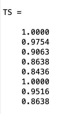
The vector of normalized inverse cube tandem finishing times for these two races is then
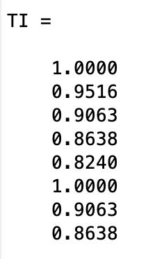
There are two ‘1’ values in this vector; each corresponds to the fastest finishing time in the two races, normalized to one hour. The numbers after these are ordered from fastest to slowest in each race. Once again, the other values are smaller because we are taking the inverse of their cube, which will always be less than one since the times of the corresponding paddlers is slower (e.g., larger) than the winner of each race.
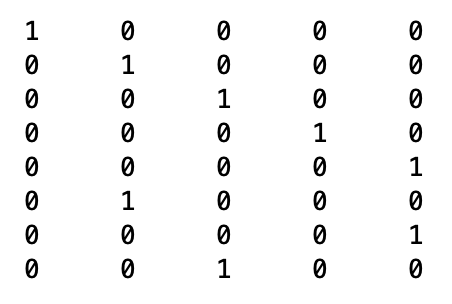
We’ve used the first race to “name” our paddlers Paddler 1, Paddler 2, etc. This means that Paddlers 2, 6, 8 and 10 did not participate in the second race. The matrix M is then
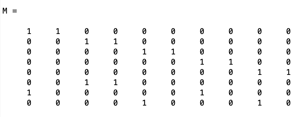
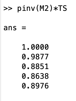
For convenience, we used the first race to establish a one-to-one correspondence between each member of the tandem teams and their results, ranked by finishing times.[8] This is embodied in the first five rows of the matrix, which looks a bit like the identity matrix save for the repeated ‘1’ entries; this reflects how we once again rank-ordered the timing vector y. The next three rows in M show that only six of the original ten paddlers participated, and their relative tandem finishing positions are reflected in the positions of the non-zero elements of the lower 3-row submatrix. Taking the pseudo-inverse of this matrix and multiplying it by the matrix of normalized inverse cube tandem finishing times yields the relative power values for these ten paddlers:[9]
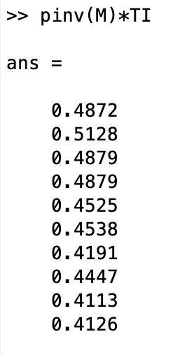
Even though Paddler 2 didn’t participate in the second race, they have the highest relative power because they finished higher than all other paddlers in the first race save their partner. Their partner, Paddler 1, dropped in rank because of their 2-minute normalized time lag compared to the winners of race 2, who as a tandem pair only trailed the leaders in the first race by one minute (normalized time). This reflects how the power ranking scheme reflects finishing times rather than finishing position, weighted using results from all races.
Notice how the sum of Paddlers 1 and 2’s the relative power equals one. This is because their sum equals the normalized (e.g., scaled) power in the hull, and as we learned from our analysis Paddler 2 has greater relative power than Paddler 1. For this model the “best” power for a hull will always equal one. Keep this in mind if you wish to merge tandem and solo race results.[10]
Paddlers 3 and 4 have the same power rating because they paddled together as a tandem in both races. If a team paddles together in all races there is no way to rank them individually; their power ratings will be the same since there is no basis for treating them differently.
If there is no common paddler between these two races the results will not reflect relative power across all paddlers. There has to be some overlap in participation between races in order to develop these relative power rankings.
You can gain insight into how well the model is working by computing the rank of the matrix M, as well as its condition number. Note that you can compute the pseudo-inverse of ill-conditioned matrices, and gloss over gaps or weaknesses in the data set.
CONCLUSIONS
In this installment of the Science of Paddling series we’ve considered a time-based rather than a finishing order-based method for ranking paddlers. The method relies on some basic physics (which we know works), careful bookkeeping of race results, and an analysis package like Matlab or R that can manipulate matrices and compute pseudo-inverses. Simple examples were presented for solo and tandem paddlers. The results are not actual paddling wattages, but normalized (e.g., scaled) relative power values.
Note that this model makes no distinction between men’s, women’s, or mixed tandem teams. Relative power is based on relative finishing times only and does not reflect any time bonuses that might be introduced in race series scoring system, including time bonuses based on age. If you wish to include any of these adjustments, you need to appropriately scale normalized finishing times using the multiplicative parameter
I’m sure some of you have been figuratively raising your hands, wanting to ask, “What about drafting and pack riding? How does your method address that?” Well, it doesn’t. What are the alternatives? You can either use this method for time trials only, or just put folks on an erg in a lab to directly measure paddling power.
Perhaps the more fun approach to address the “what abouts?” is to incorporate more race results, over different courses with different water and weather conditions, which by chance may include some different tandem pairings and novel pack groupings. With enough results this will level out results that depend upon how one race unfolded. Further, if one were to employ this approach for a season’s race series, it makes sense to require that paddlers participate in a minimum number of races to be ranked. This will only serve to improve the resulting power rankings.
REFERENCES
George Forsythe, Michael Malcolm, and Cleve Moler, Computer Methods for Mathematical Computation, Prentice-Hall Series in Automatic Computation (1977).
Forman Acton, Numerical Methods That Usually Work, Harper & Row (1970).
© Shawn Burke, 2021, all rights reserved. See Terms of Use for more information.
v1.0
- In what follows we implicitly set D to 1, like “one course length.” Since all finishing times are scaled w.r.t. a one-hour “best” time the particular value of D isn’t important. ↑
- We’ll revisit this later when considering time bonuses and hull handicapping. ↑
- You can choose any time you wish, like 13 fortnights or 13.4 billion years. One hour is just convenient. Whatever you choose be sure to use it for all races in a series. ↑
- The identity matrix I is a square matrix with 1’s along the diagonal, and 0’s everywhere else. It is the matrix equivalent of the number 1. And like the number one, if you multiply a matrix times the identity matrix you get back the original matrix. Note again that MM+ acts like the identity matrix, but is not the identity matrix. ↑
- By definition, having more results than paddlers is an over-determined system. ↑
- This is merely a convenience for this illustrative example. In practice, all you have to do is careful bookkeeping to ensure accurate mapping between race time results and paddlers. ↑
- Note that these values are not actual wattages, but instead represent relative power among participating paddlers. ↑
- See footnote 6. ↑
- Note that these values are not actual wattages, but instead represent relative power among participating paddlers. ↑
- This also suggests that relative power might be employed to estimate relative finishing times for prospective races, mixing and matching various tandem pairs. A topic for future work. ↑