by Shawn Burke, Ph.D.
Introduction
I’m a dinosaur. I prefer to derive solutions to physics problems whenever I can rather than simulate them. Even when I can’t find a closed-form solution – a solution that can be written down using pencil and paper – I look for limiting cases. What happens when one variable is large, or small? What happens when the hull/paddler/water system approaches steady-state behavior? I’ve found that these investigations provide insight across hull types, paddles, and paddling disciplines. They are not merely special cases.
In graduate school I witnessed the introduction of widespread numerical simulation into the undergraduate engineering curriculum. Some faculty members argued that one day students would no longer need to build hardware prototypes or conduct experiments. All experiments would be digital simulations. Like my dinosaur-hood, this too is an extreme. I found the lab students I taught benefited from hands-on experience with hardware, sensors, signal conditioning electronics, and data acquisition systems – some of which were cutting edge and employed digital technology. You appreciate the limitations of simulation, and your incomplete understanding of calculus, when you witness integrator wind-up firsthand.[1]
Is there a middle ground between simulation and dinosaur-hood? Sure, just master both skills. Or better yet, work with hardware to develop what my undergraduate professors called “engineering judgment,” study engineering, minor in applied mathematics, and get a degree in computer science. I can already hear the groans.
In this installment of the Science of Paddling we’ll dip our toe into simulation, while keeping our heads out of the digital clouds and firmly rooted on the water. Our model problem is the solo canoe who’s drag coefficient was measured in Part 14: Kind of a Drag. We’ll consider various paddling force profiles to determine their impact on how this canoe – or rather, this canoe model – gets off a race starting line. Which is better: short choppy paddling strokes or long strokes? Does increasing paddle force over the first few strokes get the hull up to speed faster, or not?
The Governing Equation
We can develop a mathematical model that relates the paddling propulsive force Fp to the drag force in terms of canoe speed v using Newton’s Second Law. Newton requires the sum of all forces acting on the hull to equal the total mass of hull plus paddler times the hull’s acceleration. Including the drag force, which we showed in Part 26: Waking Up was proportional to speed squared, the Second Law yields
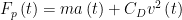
In this equation m is the mass of the hull plus paddlers and gear, while CD is the hull’s drag coefficient. The drag coefficient is specific to the hull’s shape; different hulls have different drag coefficients. The dependent variable a represents the rate of change of the hull’s velocity, otherwise known as its acceleration.
This equation is called a governing equation. Solve it, and you can predict the canoe’s speed v as a function of time t given the drag coefficient CD and the propulsive force Fp.[2] Note that this is a very simplified model of the moving hull. For example, it does not address the hydrodynamic effects of roll, pitch, or yaw, which all impact performance. Keep this in mind as we interpret solutions to the governing equation. Try not to read things into the model that aren’t there!
The governing equation looks unassuming enough. However, owing to the velocity squared term it’s a nonlinear differential equation. For those of you keeping score at home, it’s a Ricatti equation. For most propulsive force profiles Fp, the Ricatti equation does not lend itself to a closed form solution. Bummer!
Our governing equation does admit numerical solutions. To compute one, we’ll introduce a teeny bit of calculus. The hull’s acceleration is the time rate of change of its velocity, otherwise known as the velocity’s time derivative. Acceleration can be written as

The derivative notation d/dt means “rate of change with respect to time.”[3] This notation lets us rewrite the governing equation as
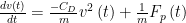
If we know the initial speed v0 at a start time t = 0 , plus the propulsive force over time and the constants, this is an initial value problem that lends itself to an iterative numerical solution.
Simulation Model
Let’s assume that the hull’s initial speed is zero. We’ll use the drag coefficient for a solo hull computed from our field tests outlined in Part 14: Kind of a Drag, plus a mass of 109 kg for the combined hull, paddler, and gear. We’ll represent the propulsive force as we did Part 11: About the Bend. As a baseline we’ll use a 1-second stroke duration, which corresponds to a 60 strokes/min cadence. We’ll initially assume the stroke has a 70% duty factor. This means the power phase lasts 70% of the stroke duration, or 0.7 seconds.
All simulations were conducted in Matlab. We used Matlab’s ‘ode45’ solver, which employs an explicit 4th-order Runge-Kutta method.[4] The initial time vector ran from 0 to 60 seconds in 1 millisecond increments. The ode45 solver internally adapts the time step as needed to address tolerance and solution convergence.
Results
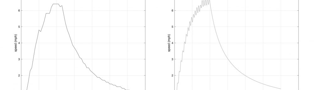
We begin by comparing the experimental hull speed data with our simulation model. As you’ll recall, we brought the C1 up to speed, then let it coast. This let us use the solution to the homogenous governing equation during the coasting phase to compute the hull’s drag coefficient. You can compare experiment and theory in Fig. 1’s two plots.
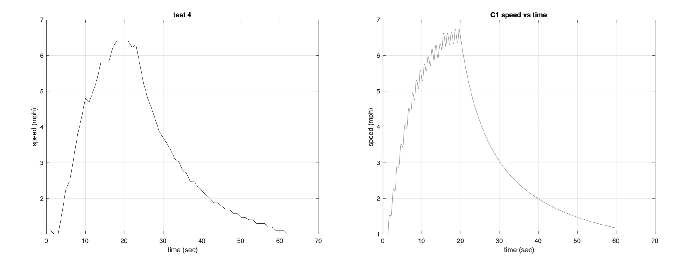
Figure 1: C1 experiment and simulation.
The GPS used in the field to acquire speed data digitized at one sample per second. Consequently, the finer details of hull motion are lost, and the data at lower speeds is a bit chunky. However, the general trends seen in the experimental data are reflected in the simulation. The average speed rises like it would for an over-damped system, then drops inversely as time during the coast. Since there was no way to measure propulsive paddle force during the field tests I chose a peak force amplitude for the simulation that matched (as best I could determine) the steady-state hull speed just prior to the coast phase.
You can see a “close up” of the simulation data in Fig. 2. As the simulated hull approaches its cruising speed the quadratic drag force increases, and the “hull” displays speed surges that are rapidly damped by this drag. At lower speeds the drag force is lower as well, hence the speed surges there don’t damp out as quickly. At low speeds the hull appears to “ratchet” up the drag curve. If the simulated propulsive force isn’t turned off at t = 20sec the “hull” speeds along at its average cruising speed, with speed oscillations at each stroke. Not surprising (and kinda boring).
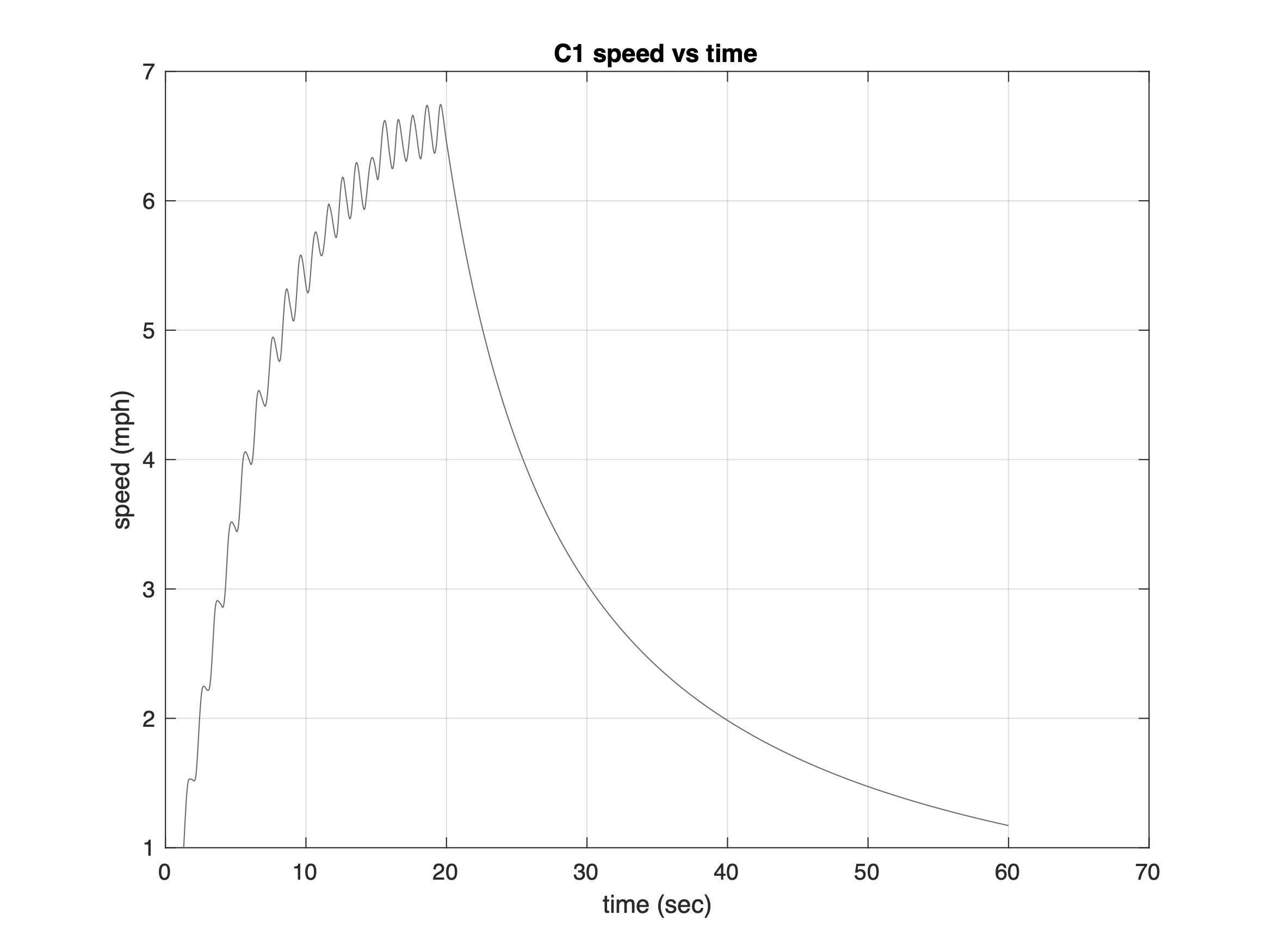
Figure 2: C1 simulation data.
Now I’ve seen top-end racers with vastly different paddle strokes. A friend of mine (who shall remain nameless) has a fast, choppy stroke, while I know another paddler who employs longer strokes. Yet they’ve finished neck-and-neck at numerous races. So I investigated two radically different propulsive force profiles. The first, which is our baseline, has a one-second stroke duration and 70% duty factor. The second has a two-second stroke duration (30 strokes/min cadence), along with the same 70% duty factor. These two force profiles are plotted in Fig. 3. A 30 strokes/min cadence is certainly slow for racing. But the goal was to see how a longer stroke, with all other factors held constant, might impact speed.
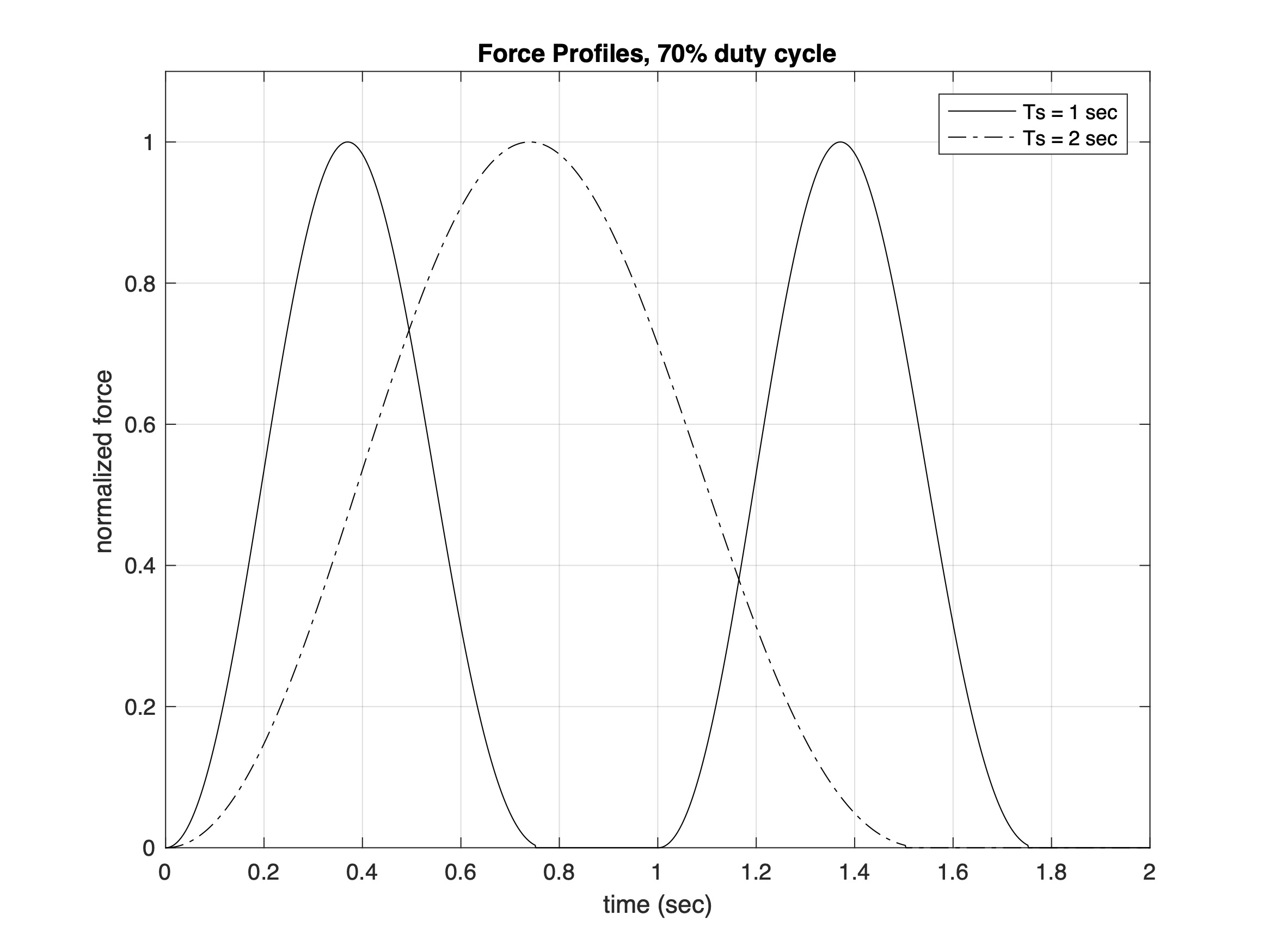
Figure 3: Normalized propulsive force profiles for two cadences.
The simulated hull speed curves for these two force profiles are plotted in Fig. 4.
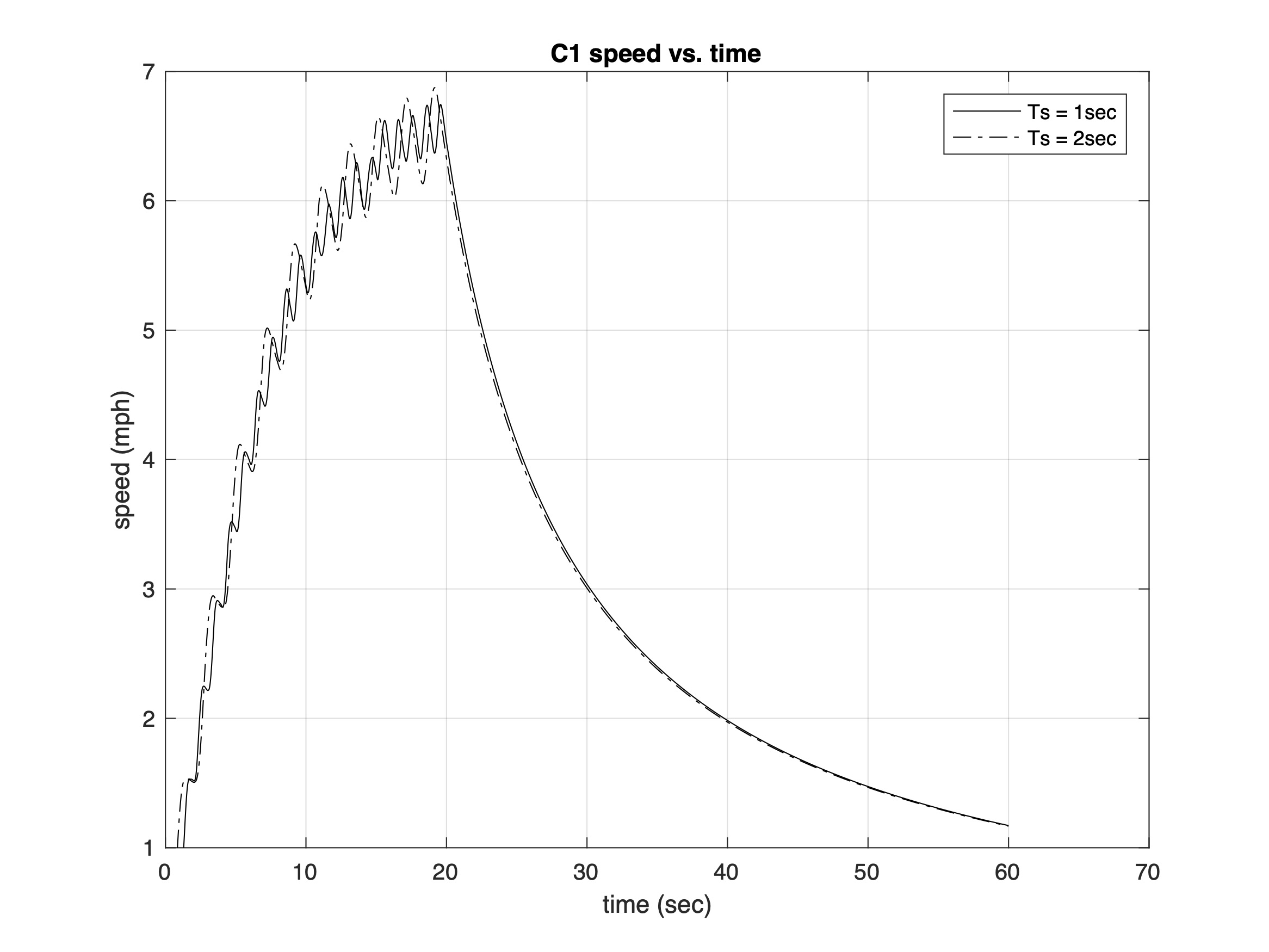
Figure 4: C1 simulation data for fast and slow cadence force profiles, 70% duty factor.
As you can see in Fig. 4 the results are scarcely different at all. The lower cadence results display speed oscillations at half the rate for the faster cadence. But aside from that the average speed trend through these two cases is essentially identical.
Why does this happen? Recall from Part 25: Impulse Part 1, and Part 33: Impulse Revisited that a hull’s momentum – and thus its speed – are driven by the impulse that the paddle/water system imparts. We showed that impulse is proportional to the area under the force versus time curve. The two force profiles in Fig. 3, corresponding to 60 spm and 30 spm cadences, have identical areas under their curves. This is because they both use the same generative model and have the same duty factor.
There are two notable results from these simulations. First, it doesn’t matter whether you have a fast stroke or a slow stroke if you apply the same impulse. Your body may be better suited to a cadence, so work with that. And second, Figs. 3 and 4 show that a model derived from Newton’s Second Law, and a model developed using conservation of momentum, yield the same result. Since we’re operating in the world of classical mechanics this had better be the case! But if you’re new to physics you might wonder why I might choose one method of attack versus another. The reason? Convenience. They both describe the same reality, as (fortunately) demonstrated by our results.
So, if stroke cadence won’t get a C1 up to speed faster, what will? I then looked at the role duty cycle plays. Using our baseline paddling model with a 60 strokes/min cadence I compared 60%, 70%, and 80% duty factors. Recall that a higher duty factor means a faster the recovery; the stroke’s power phase is longer as a percentage of the total stroke duration. These three force profiles appear in Fig. 5.
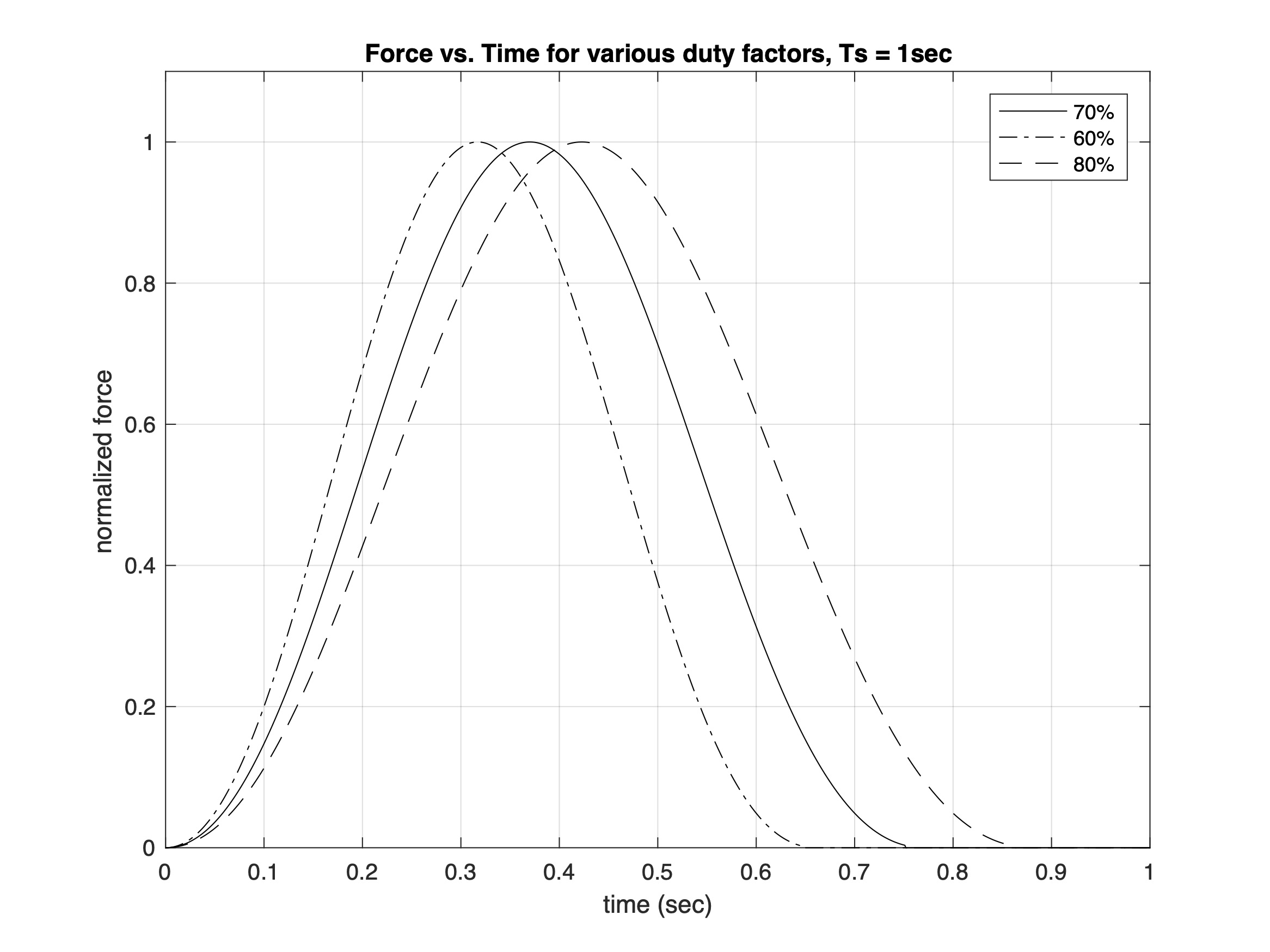
Figure 5: Normalized propulsive force profiles for three duty factors.
The simulation results for these three propulsive force inputs are plotted in Fig. 6. The higher duty cycle force profile yields a greater top speed before the coast, while the lower duty cycle profile yields a lower top speed. This isn’t surprising when we consider the impulse imparted by each profile. Since the stroke’s length is the same in all three cases the only differentiator is the duty cycle. For a fixed cadence a higher duty cycle provides more impulse, yielding greater hull momentum and thus speed. Yay – physics works! But notice that all three cases come up to speed at about the same time. Higher duty cycle yields a greater top end. And that top end occurs about the same time for each.
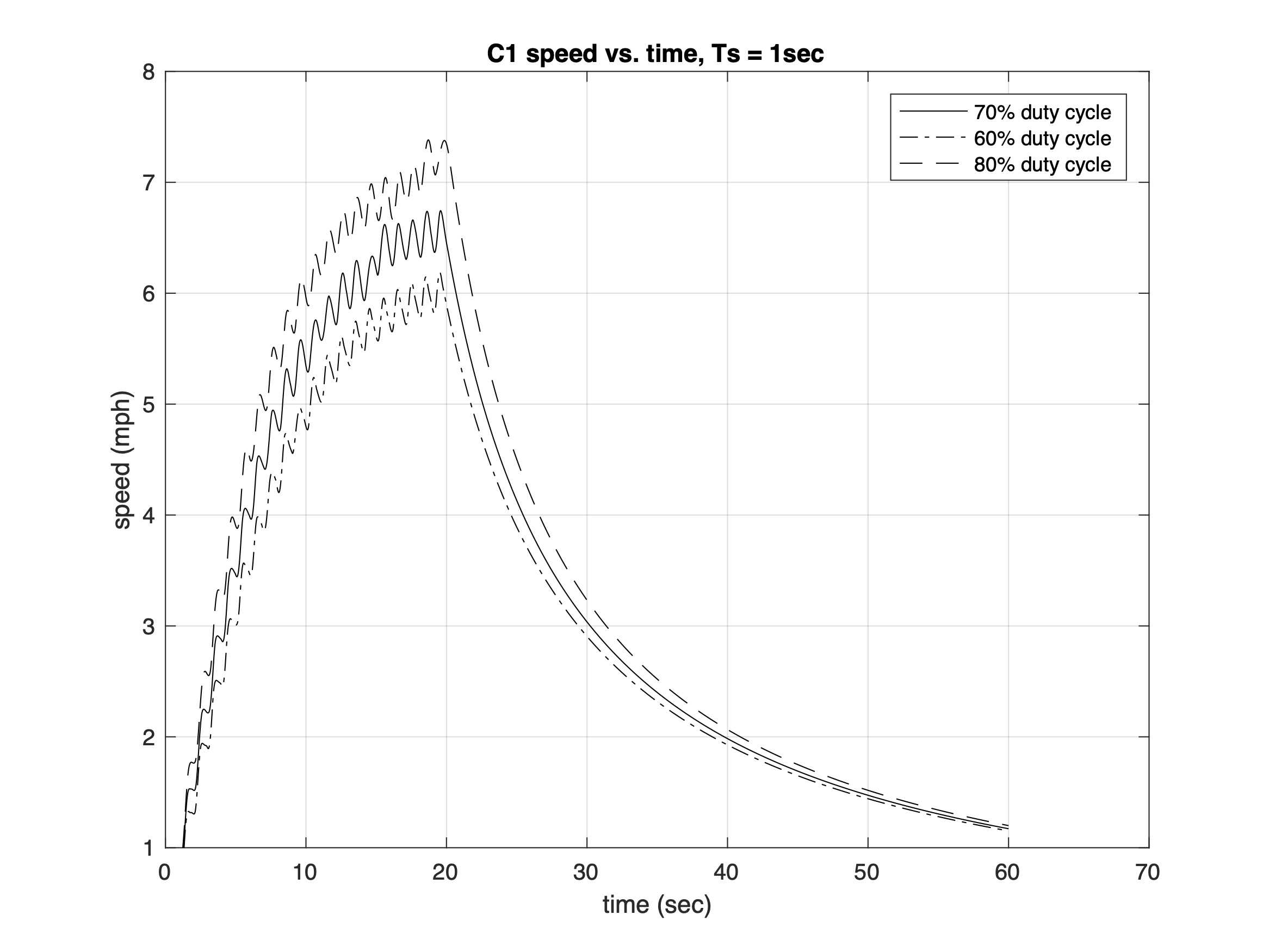
Figure 6: C1 simulation data for force profiles having various duty factors.
What might get a hull up to speed faster? Many of us apply greater force over the first few strokes as we get up to speed. Our propulsive force tapers over several strokes, whereupon we engage our steady-state paddling mechanics. To capture the flavor of this I simulated a force profile with varying peak force over the first ten strokes, as depicted in Fig. 7. The first stroke is done at 150% of the steady state peak force. The force curves for each stroke taper linearly until t = 10sec. Thereafter they are identical to the Ts = 1 sec stroke in Fig. 3.
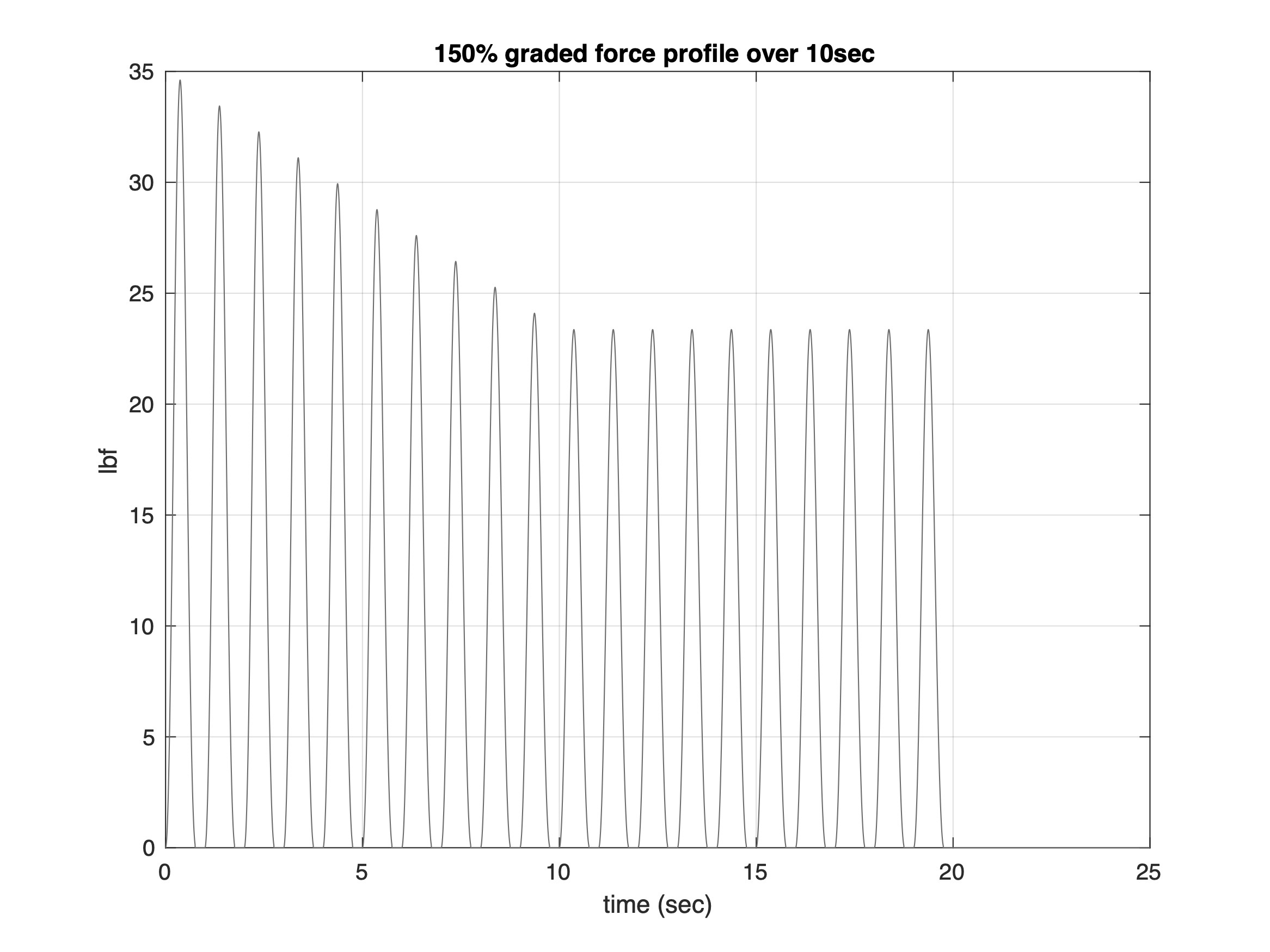
Figure 7: Variable propulsive force profile.
It will come as no surprise that harder initial strokes bring the simulated C1 up to speed faster, as shown in Fig. 8. Despite having the same cadence, the stronger initial strokes in the graded profile get the simulated hull out of the hole faster, ratcheting up the drag curve more quickly owing to each stroke’s greater impulse than the baseline force profile’s.
You could combine effects, and both grade the stroke force over time, and grade the stroke duration over time (e.g., initially slower strokes transitioning to a faster steady-state cadence). That result is left to the reader to investigate. But considering what we know about physics, we can predict what the result will be. If the force profile entails greater impulse, you’ll go faster. If it entails greater impulse over a single stroke than over others, you’ll speed up more quickly.
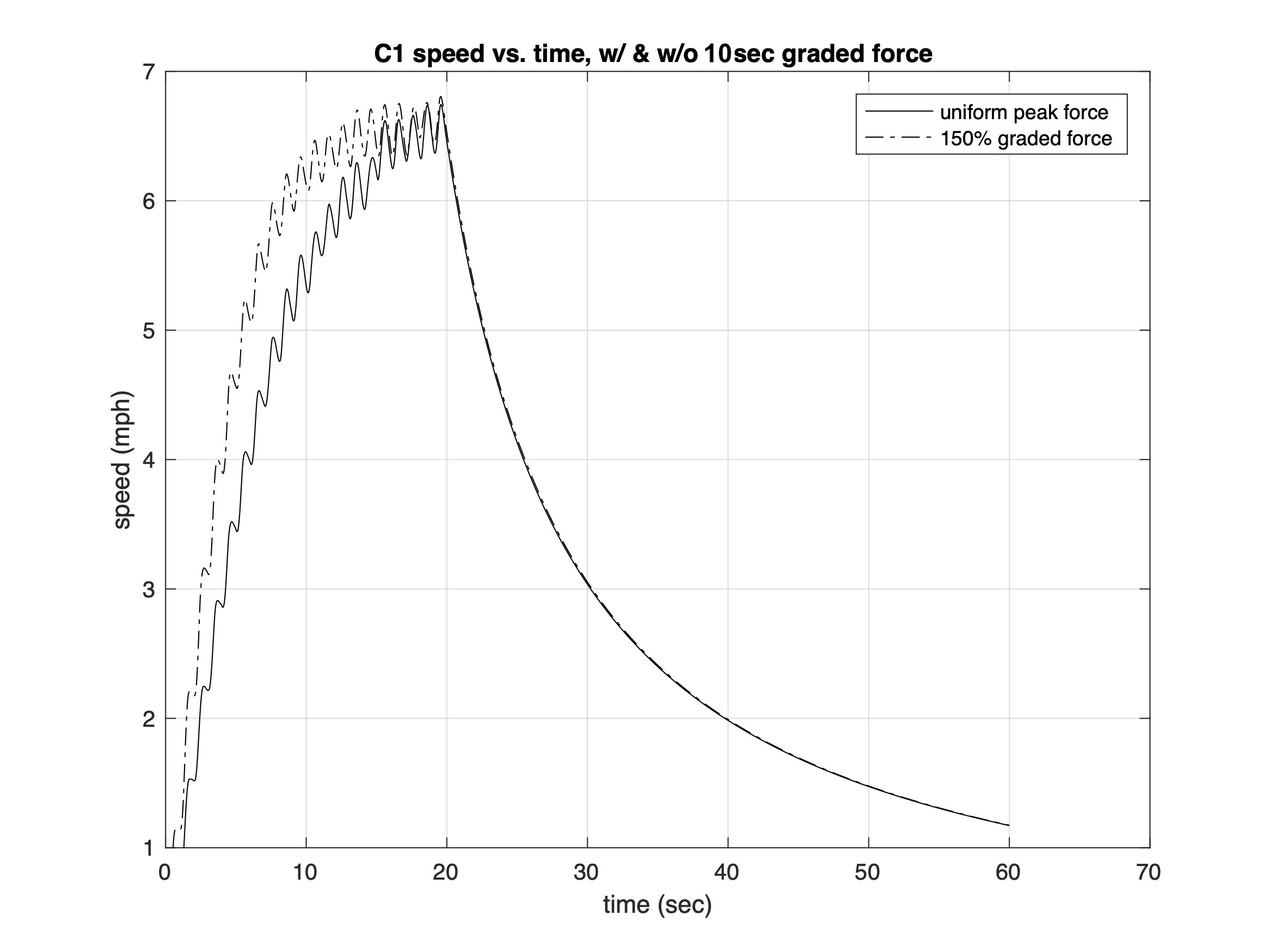
Figure 8: C1 simulation data for uniform and graded force profiles, Ts = 1sec.
Conclusions
In this installment of the Science of Paddling we’ll dipped our toe into simulation. And it didn’t hurt a bit! Our simulation model was based the solo canoe studied in Part 14: Kind of a Drag. We investigated various paddling force profiles to determine their impact on how this canoe – or rather, this canoe model – gets off a race starting line.
We found that faster and slower paddling cadences did not impact the simulated hull’s speed versus time curve for a given force curve and duty cycle. This reflects the role impulse plays – the area under the force curve. If the impulse is the same, the hull’s resulting momentum and thus speed will be the same. Changing the stroke’s duty factor – the percentage of the stroke were the paddle provides propulsion – changes the simulated hull’s top end speed. Greater duty factor means greater impulse; the result was not surprising. And finally, you’ll get off the line faster by employing more powerful strokes at the start for a given stroke rate. Again, it all comes down to the impulse you impart through the paddle.
Perhaps this article’s greatest value is in how it ties together Newton’s Second Law and momentum conservation. Some readers may be more comfortable starting from F = ma. Other times it’s advantageous to start from momentum conservation. But the results are (fortunately!) the same.
References
F. Acton, Numerical Methods That (Usually) Work, Harper & Rowe, New York NY, pp. 129-156 (1970).
G. Forsythe, M. Malcolm, and C. Moler, Computer Methods for Mathematical Computation, Prentice-Hall, Englewood Cliffs NJ, pp. 121-146 (1977).
© 2022, Shawn Burke, all rights reserved. See Terms of Use for further information.
- Integrator windup happens when you digitally integrate a signal. For example, we know that acceleration is the derivative of velocity, so velocity is the integral of acceleration. Many newbies then conclude that you can integrate an accelerometer signal and presto! You’ve got velocity. But if the accelerometer, its signal conditioning electronics, or your digitizer’s front end have a DC offset you get to witness the time integral of a constant. Over time the integral trends toward infinity. Practically, the signal will grow until it exceeds some component’s dynamic range and saturates the electronics and/or the signal’s digital representation. Fun times! ↑
- Or rather, you can derive a solution to the mathematical model that hopefully represents reality! ↑
- Newton would have called it a fluxion. ↑
- See, for example, F. Acton, Numerical Methods That (Usually) Work, Harper & Rowe, New York NY, pp. 129-156 (1970), or G. Forsythe, M. Malcolm, and C. Moler, Computer Methods for Mathematical Computation, Prentice-Hall, Englewood Cliffs NJ, pp. 121-146 (1977). ↑