Part 14: Kind of a Drag

by Shawn Burke, Ph.D.

INTRODUCTION

I’ve often wondered if the performance of a canoe, kayak, or SUP can be characterized by just a few numbers. Like the information printed on a new car’s window sticker. We see ads for various hulls touting their performance in waves, wash, shallow water, deep water, following seas, etc. There are accolades like “great” and “fast” and “handles X with ease” for whatever ‘X’ is. OK, but “great” and “fast” and “with ease” compared to… what? Wouldn’t it be helpful, for example, if “fast” was expressed on a quantitative scale running from 1 to 100?

Now granted, this kind of perspective is itself limiting. I’ve climbed into hulls that I couldn’t keep upright. So the fact that they’re also fast is largely irrelevant if I can’t handle the boat! There are indeed qualitative, paddler-specific characteristics that factor into hull selection and use. But still… I’d like a number, please. If for nothing else than to convince myself that a new hull I’m buying is actually a step up from what I already have.

Since this is a Science of Paddling article you won’t be surprised to learn that physics provides a number that may be useful in characterizing and even comparing hulls. In addition, we will explore the conundrum raised in the last article: do physics-based models actually represent reality? And equally as important, can we construct a simple test that anyone can perform in the field – or actually, on the water – to validate our models, and in the process characterize our own hull(s)? For those of you who don’t wish to read any further (or have any fun), the answer is… Yes! And it all hinges on the gremlin that keeps us from paddling faster: drag. So if you’d like to delve deeper, and learn how you (yes; you!) can “do some science” the next time you’re on the water, read on.

ABOUT THAT MODEL

As we learned in Part 1, the dynamics of a hull in motion in one dimension is modeled using a balance of forces: the propulsive force F exerted by the paddler(s), which via Newton’s second law is proportional to the combined mass m of the paddler(s), hull, and gear times their acceleration; and a drag force that opposes their efforts, as depicted in Figure 1:

$F-{{C}_{d}}{{v}^{2}}=m\frac{dv}{dt}$

Here, v is the hull speed, and dv/dt is the time rate of change of that speed, otherwise known as acceleration. The drag force opposes the propulsive force, hence the minus sign. As discussed in Part 1 the drag force is modeled as proportional to the square of the speed. Note that our model omits the effects of wind and current; these can be included, but for simplicity we’ll leave them out. Since our analysis is limited to one spatial dimension all quantities are scalars. The propulsive force F and the speed v also vary with time t; the other terms in the equation are constants.

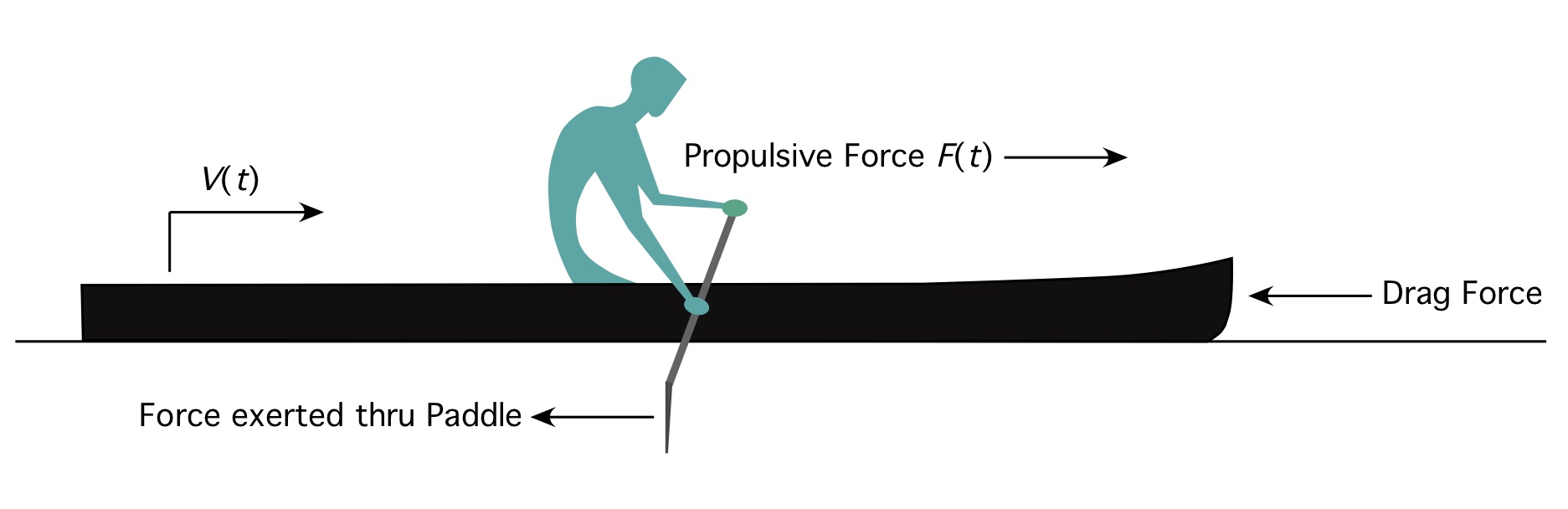
Fig. 1: Idealized paddler and dynamics elements^[1].

As we noted way back in Part 1 the drag force on a canoe, kayak, or SUP hull can be characterized – subject to a few assumptions – by a single parameter, the so-called Drag Coefficient, denoted as C_d. The Drag Coefficient is a property of the hull and how it sits in the water^[2], plus any form drag introduced by the paddler’s body’s wind resistance.

The governing equation above has the form of a so-called Ricatti equation, and can be solved in closed form (e.g., you can write down the solution for the speed v on a piece of paper, rather than having to resort to numerical simulation) for certain force functions F. If instead we consider what happens when the paddle force is zero, such as when you stop paddling, our governing equation reduces to a simple first-order nonlinear ordinary differential equation:

$-{{C}_{d}}{{v}^{2}}=m\frac{dv}{dt}$

So if a hull is moving with a known speed V₀, then at time t = 0 one stops paddling^[3], it’s fairly easy to solve this equation. The so-called “homogeneous” (zero force input) solution for the speed v is derived in the Appendix (for those of you who like extra fun), and takes the remarkably simple form

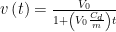
$v\left( t \right)=\frac{{{V}_{0}}}{1+\left( {{V}_{0}}\frac{{{C}_{d}}}{m} \right)t}$

The reader can verify that this is correct by substituting the solution into the homogeneous governing equation of motion. Or you can take my word for it. Qualitatively the expression for speed v(t) makes sense; when time t = 0 the hull speed equals V₀; check. And as time t increases the denominator gets larger, so the speed v decreases over time; check. This reflects to our experience paddling canoes, kayaks, and SUPs. But does it accurately reflect what happens in the real world, with real hulls? Hang on; we’ll get to that.

The homogeneous solution requires that you know the initial velocity V₀, which can be measured, for example, using a GPS receiver. It also requires that you know the combined mass of the hull, paddler(s), and gear. A bathroom scale (or two) will suffice to measure this. So the only thing standing between you and knowing the speed as a function of time is the Drag Coefficient C_d.

So where to you get the drag coefficient? Well, you visit the website of your favorite canoe, kayak, or SUP manufacturer, and you look it up! Wait; what? Can’t find it there? Hmmm… What’s to be done?

Well, naturally, you go onto the water (or as I refer to it, The Lab), conduct tests, acquire data, then go home and crunch the numbers in order to compute the Drag Coefficient. I mean, who wouldn’t jump at the opportunity? You see, the model motivates the tests to be conducted. The solution to the homogeneous governing equation relies on measurable quantities (the initial velocity V₀ and the combined mass m). It is based on a scenario where you (1) paddle to bring the hull up to speed, then (2) stop paddling and coast. If you measure the speed v as a function of time while doing this, you can plot this data, compare it to the model’s prediction, and use that comparison to deduce the Drag Coefficient. And your hull will be characterized.

Let’s try it and find out.

TESTING: ENTER… REALITY

In order to get test data I first needed to choose a hull. I chose to paddle my Savage River D-IIx USCA C-1 solo canoe; you can use any hull you want as long as you follow the test protocol outlined below, including using tandems (or even C4s – that would be fun!). During all tests I set the seat’s fore-and-aft position so that the hull had a neutral static trim. While it might be interesting to parametrically study the influence of trim, I decided one configuration was sufficient since the point of this exercise was to determine if all of this model-test stuff actually worked.

I also needed an appropriate venue. Since I wanted the data to reflect the inherent hydrodynamic characteristics of the hull, and not to be influenced by shallow water effects, the water at the test site had to be as deep as half the length of my hull; see The Science of Paddling, Part 4: Shallow Water for why. Since my C-1 is 18’ 6” long this meant I needed a course that was at least 9’3” deep. In order to get the hull up to speed then coast I estimated the test course needed to be about a tenth of a mile long. A requirement of no current indicated that a lake or pond with the appropriate depth would be the right choice. And finally, the requirement of no wind at all meant I had to conduct tests very early in the morning; this is a one more reason why I went solo!

Fig. 2: Test site at 5:30am.

After searching fishing depth maps for lakes and ponds in Eastern Massachusetts I was surprised to see that a portion of a local pond met all of my criteria. It was even better that the pond is only a short drive from my house; I’ve used it often for interval and other short-duration workouts. Field Pond it was! You’ll find a depth map below; the test course is marked on the map. With a depth ranging from 8’ to 11’ over the test course my depth requirement was met. Barely. The test area had an open view of GPS satellites, and tests were short enough that a single GPS satellite constellation could be in view at all times so that there wouldn’t be any “jumps” in position if the constellation of satellites changed.

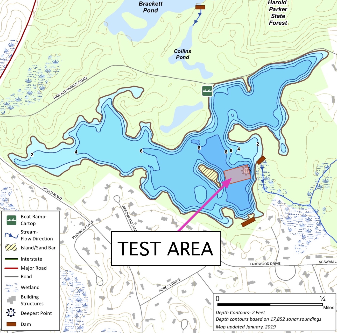
Fig. 3: Field Pond depth map and test area location. (source: Massachusetts Division of Fisheries and Wildlife)

So, paddle in hand I pushed off from the shore, fired up my Garmin Forerunner 920xt GPS receiver and waited for it to lock on to the satellites, warmed up a bit, and made my way to the test area. The morning was dead calm, and aside from a fisherman I saw on shore I had the venue to myself. Recent rains had topped up the pond nicely. Tests were conducted as follows:

After a few practice runs a series of eight (8) test runs were conducted, each lasting approximately one minute and ten seconds (1:10) and covering about one tenth (0.1) of a mile.
Test runs were done in alternating directions to eliminate any systematic errors that only testing in one direction might introduce.
Data was taken using the Garmin Forerunner 920xt, set to acquire one datum set (time, position, speed) per second. (Note that many wrist-mounted sports computers have GPS receivers that employ “smart” data recording. Smart data recording often entails taking fewer data points, further apart in time, and at non-regular time intervals.)
For each test I began from a stationary position, the GPS receiver was started, and the hull was brought up to speed over 15 – 20 seconds.
Once up to speed, paddling was halted, I sat upright just as if I were paddling, and the paddle blade was feathered so as not to introduce blade face wind drag into the data.
Once the GPS showed 0 mph speed the GPS receiver was stopped, and data was saved.

The first thing I discovered is that it’s very hard to set and maintain the hull perfectly vertical, with no roll or wobble whatsoever, when it is coasting at low speed. It was also easy to stop paddling and have the canoe immediately start carving a turn. Or start turning about half way through the coasting phase, as shown in Fig. 4. In Fig. 4 the canoe was traveling right-to-left; the red trace reflects the GPS track. Note that this carving occurred toward both left and right; there was no consistent direction that could be attributable to, say, hidden currents or an undersea monster.

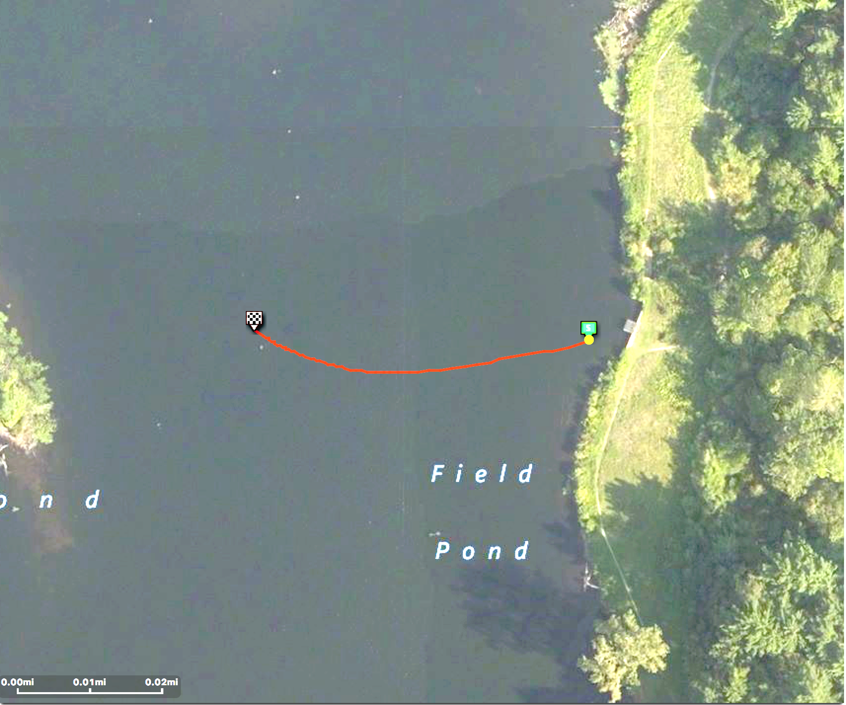
Fig. 4: GPS track, Test 1.

A representative trace of speed vs. time is shown in Fig. 5. Since the GPS receiver is acquiring and storing data once per second you don’t see any detail in the trace that would indicate the smaller speed variations associated with each stroke prior to the coasting phase. This would require a different GPS receiver and software capable of acquiring and recording data 5-10 times per second, which I do not have. Fortunately, the coasting phase velocity trace is a smooth curve, as seen in Fig. 5, so the once-per-second data recording is sufficient to capture the dynamics there. Also, this receivers speed data below ~1 mph is suspect; note the immediate jump in the data at the start. Above 1 mph GPS data for this receiver is probably accurate to about a 1-2 tenths of a mile per hour at best. Fortunately, I had a good lock on the satellite signals, and the data looks reasonable in light of prior experience.

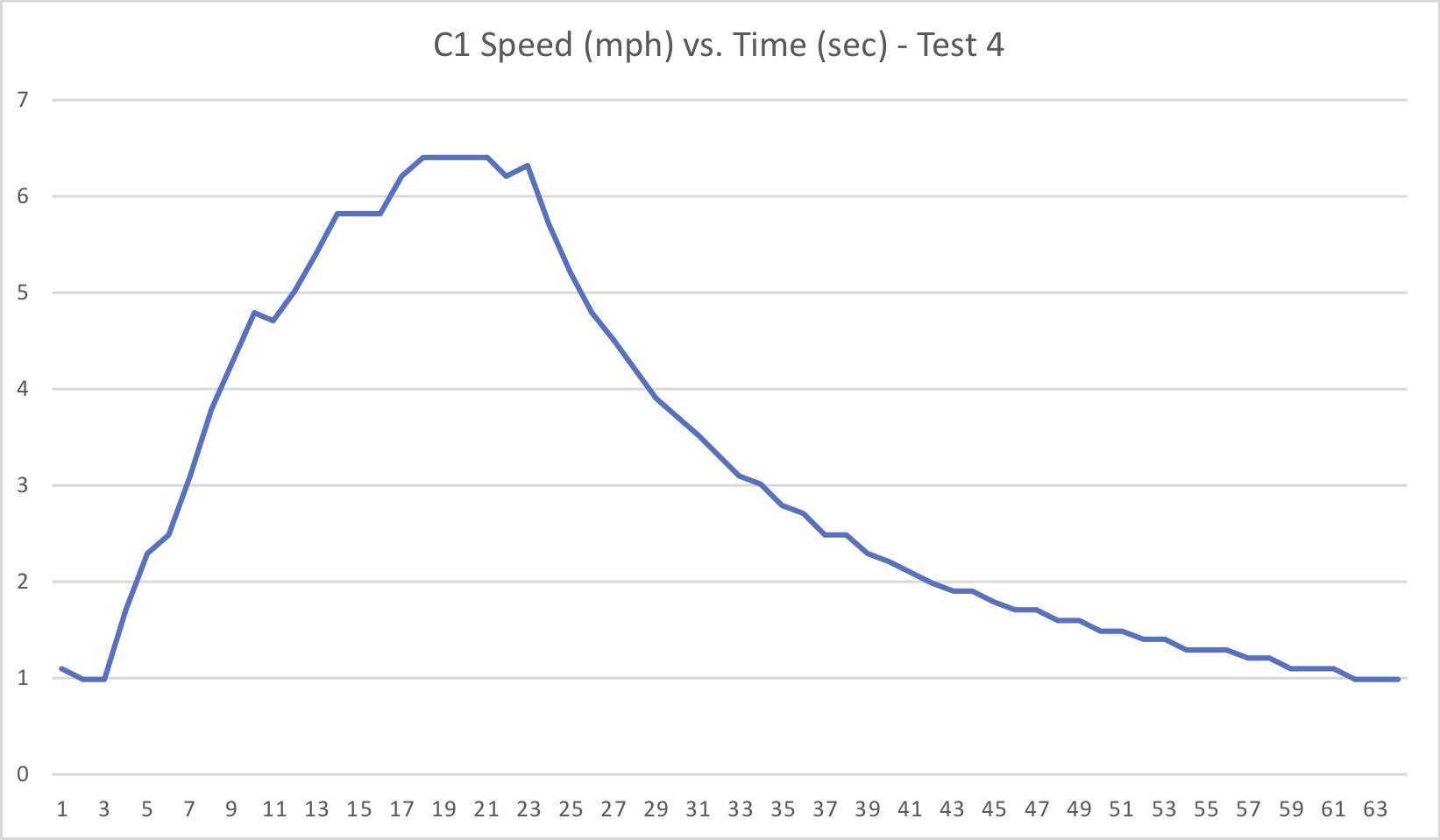
Fig. 5: Representative speed vs. time data set (Test 4).

After acquiring data from eight runs I did a workout (since I was already on the water), then returned to The Science of Paddling World Headquarters (aka, my office) and crunched the numbers. In reviewing the test results I learned that it was often difficult to discern from the data when exactly my paddling stopped, and the coasting phase began. In part this can be attributed to the accuracy of the GPS data points, as noted above, as well as having data sampled once per second (which implicitly assumes I stopped paddling on the second, rather than some time between whole seconds). The solution to the homogeneous governing equation requires the initial coasting speed V₀. However, the paddle force is still zero for all times after I stopped paddling – the governing equation is unforced (e.g., homogeneous). If I select any “first” data point after the hull starts to coast, the homogeneous solution applies. I need not select the exact moment paddling stops.

In order to derive the Drag Coefficient I settled on data from two consecutive runs in opposite directions, with minimal turning compared to the other test sets. GPS tracks from tests 5 and 6 appear in Fig. 6 below.

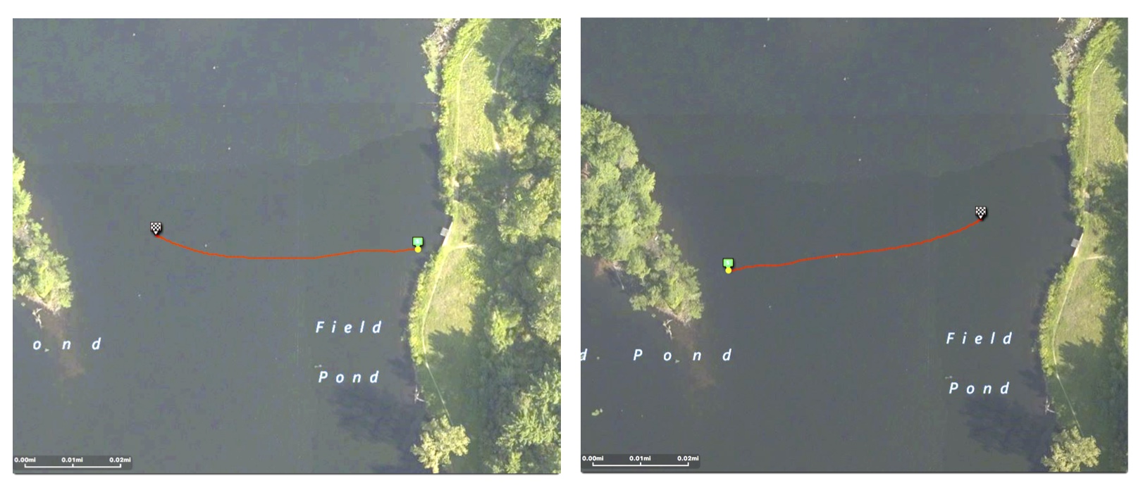
Fig. 6: GPS tracks, Tests 5 and 6.

Each data set comprises a series of data at time points t_i, where i is an index that denotes the particular data point (here, from index number 1 at the start to around 41 at the end of the coasting), with speeds at corresponding points in time v_i. The model solution produces predicted speed data at these time points, given the total mass m, the initial speed V₀, and an estimated value of the Drag Coefficient C_d. Values of the Drag Coefficient were varied in the model so as to minimize the normalized mean square error e between the test data and the model prediction^[4]. For those of you following along at home, this is expressed by

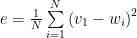
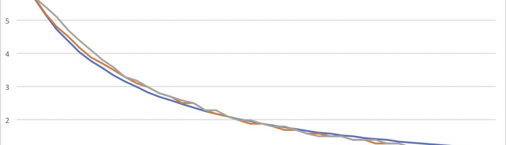
$e=\frac{1}{N}\sum\limits_{i=1}^{N}{{{\left( {{v}_{1}}-{{w}_{i}} \right)}^{2}}}$

where w_i are the speed values predicted by the model, and N is the number of data points. The comparison between speed values predicted by the model and data from tests 5 and 6 is shown in Fig. 7.

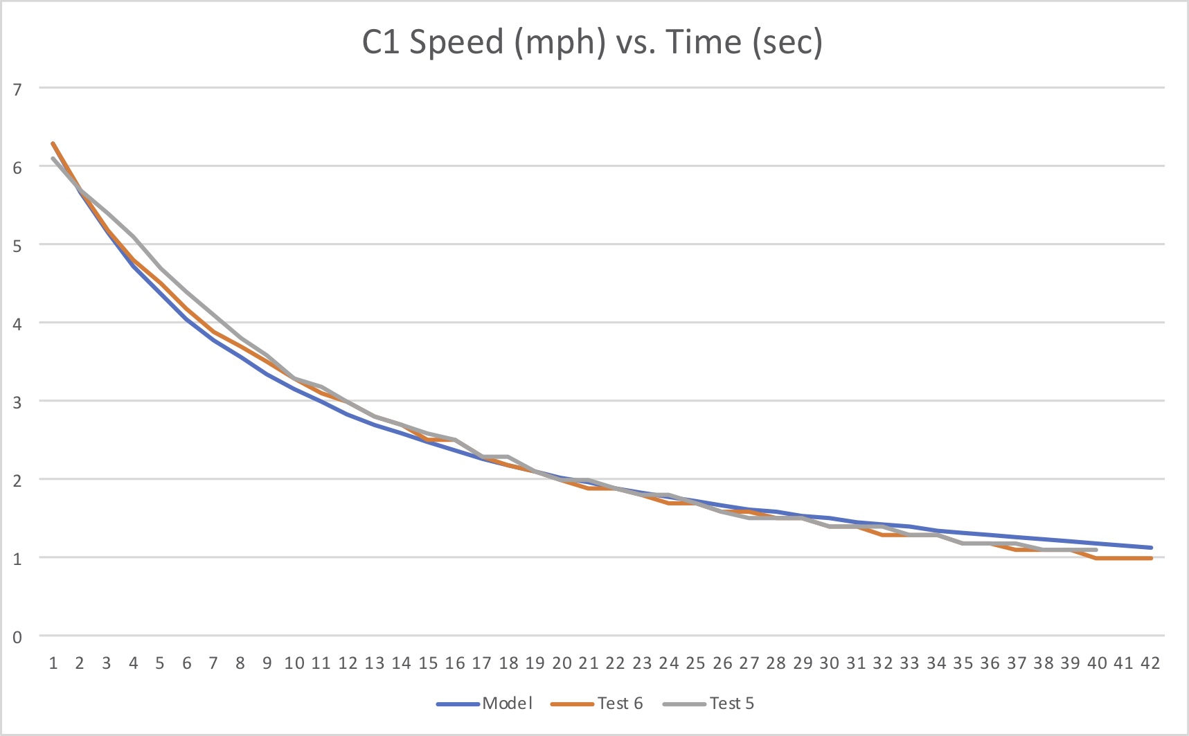
Fig. 7: Speed vs. Time during coasting phase, model vs. test data.

As seen in the figure the agreement between theory and experiment is quite good. The difference is attributable at least to assumptions inherent in the model. We have assumed that the drag force is proportional to the square of the speed, and lumped all drag effects into a single parameter. Alternative approaches have introduced additional elements in the drag model linearly proportional to the speed, or proportional to a fractional power of the speed; these might improve the model fidelity and better match the data, but would require a data regression to infer multiple drag parameters (and a more complex model that may not yield a closed-form solution). That said, our simpler model works quite well, and offers the advantage of providing a closed-form solution to the governing equation, which I always find comforting.

As to the Drag Coefficient value – you know, the stated point of this whole exercise – the mean square error was minimized for C_d = 4.2619 kg/m. I don’t expect to see manufacturers posting this number anytime soon, but wouldn’t it be fun if they did?

DISCUSSION

The test protocol laid out above can be performed by anyone if they so choose. I hope to acquire data in the near future for other hulls that I own, if for nothing else than to provide data for models that will allow me to write other Science of Paddling articles! For now that I have (or can generate) a Drag Coefficient for any particular hull, I can solve the inhomogeneous governing equation noted previously, and then run simulations to infer the role of synchronization in C2s and C4s (yeah, I’m not happy with the analysis in Part 2 either), the influence of different paddling force profiles, paddling cadence, etc. Or I may be able to use this data to qualify any new hull I might consider buying, even doing the number crunching in the field – all you need is a GPS receiver, a laptop, and a copy of Excel or Matlab.

Another application of this analysis and test protocol would be to characterize the effect varying hull trim has on drag, and to quantify the effect of shallow water and the dreaded “intermediate” depth water (aka, concrete water). Plus a whole range of other conditions.

The test method described above still needs some work. It would be good to nail down the cause(s) of why the canoe carved turns at low speeds, and do a better job at realizing straight test tracks. It would also be good to reproduce the test results on another suitable pond. And to use a GPS receiver that can acquire data faster than once per second. Perhaps the biggest open question is, how big a difference is there between Cd values for various hulls? Would the differences be lost in the noise? Hmmm… there’s always more to do.

That said, the exercise reinforced my faith in physics. The model and experimental data match remarkably well. I’m still goggled at how a classical physics model (itself a concept) and some mathematics (also conceptual) can predict phenomena in the real world. I guess Newton was right after all.

APPENDIX – SOLVING THE GOVERNING EQUATION

As derived above, the homogenous governing equation takes the form

$-{{C}_{d}}{{v}^{2}}=m\frac{dv}{dt}$

This can be re-written as

$\frac{dv}{dt}=-\frac{{{C}_{d}}}{m}{{v}^{2}}$

Define a new variable z such that

$z\equiv {{v}^{-1}}$

so that the homogeneous governing equation takes the particularly simple form

$\frac{dz}{dt}=\frac{{{C}_{d}}}{m}$

This simple derivative can be directly integrated to solve for z

$z=\frac{{{C}_{d}}}{m}t+k$

where k is a constant of integration. In terms of the speed v, this becomes

$v=\frac{1}{k+\frac{{{C}_{d}}}{m}t}$

Since at t = 0 (the start of the coasting phase) v = V₀, the constant of integration k then equals 1/V₀. Substituting into the expression for v and simplifying, the speed as a function of time during coasting is then

$v\left( t \right)=\frac{{{V}_{0}}}{1+\left( {{V}_{0}}\frac{{{C}_{d}}}{m} \right)t}$

Q.E.D.

REFERENCES

Nicholas Caplan, “The Influence of Paddle Orientation on Boat Velocity in Canoeing,” International Journal of Sports Science and Engineering, Vol. 3, No. 3, pp. 131-139 (2009).

James Buckmann and Samuel Harris, “An Experimental Determination of the Drag Coefficient of a Mens 8+ Racing Shell,” SpringerPlus 2014, 3:512.

v1.0

Note that the propulsive force is a reaction force, acting in the opposite direction of the force exerted through the paddle. This is due to Newton’s 3^rd Law (“action-reaction”). Also, the propulsive force must point in the direction of motion, otherwise it would not accelerate the hull in the forward direction. ↑
When you climb into a canoe your weight causes the hull to displace water, and pushes the keel further beneath the waterline than when unloaded. The drag force in practice reflects how the hull sits in the water, e.g. on the actual shape and volume of the hull that is in the water when paddled (and thus loaded). ↑
One of the great things about classical physics is that you can always “rewind the clock” and make the starting time equal to anything you want. Setting it to 0 is especially convenient mathematically. ↑
This is a fancy way of saying that at each increment in time the difference between the test data and the model’s predicted data was computed, then squared, then all of these squared values were summed and divided by the number of data points. Why squared? Because at some time values the test data will be greater than the model’s predicted value, while at other points it will be less, so sometimes the difference will be positive and sometimes negative. If you add positive and negative numbers they can cancel each other out, and indicate that the model fit is excellent when it clearly isn’t. The squares of the differences, however, are always positive, and their sum will always be a positive number as well, so the algorithm iterates on the value of the Drag Coefficient that minimizes this sum. One divides by the total number of data points (e.g., normalizes the data) to take into account the fact that some data sets have more or fewer data points than others. ↑