Mathematics | The Science of Paddling

by Shawn Burke, Ph.D.

OVERVIEW

Ways to cross a river in the shortest time and shortest distance are derived for various cross-stream river current profiles. These goals are shown to be mutually exclusive.

INTRODUCTION

So you’re resting in a slack water eddy along the shore of a whitewater river, wondering how to work across the current to get into the next eddy. You’re tired after a day of running rapids, and pondering, “Gee, I wonder what the fastest way to do that is?” And if you’re a nerd like me you might ask, “Can I get there in the shortest distance, too?”^[1]

Well, sure; you can do that. And whether you realize it or not you’ve posed an optimization problem. Optimization problems arise all the time in engineering and mathematical physics. They are based first and foremost on a clear, quantitative statement of the desired outcome, such as performing a task in minimum time or with minimum energy; minimizing the amount of metal waste created in forming an automotive part; optimally transmitting a weak cell phone signal in the presence of interference; etc. After quantifying the goal, the means for finding an optimal way to perform the stated task is usually posed in mathematical terms. Sometimes very, very mathematical terms involving calculus, matrix algebra, and the like. In fact, the river crossing problems posed above lend themselves quite readily to a subset of math called variational calculus.

But who needs that when you can draw pictures instead?

So in this installment of The Science of Paddling we’ll tell you a lot of stuff you already know. And skip the variational calculus.^[2] Instead, we’ll use a little geometry and trigonometry, along with vectors, to more intuitively solve the minimum time and minimum distance crossing problems for a few different cross-stream current profiles.

VECTORS

Let’s start with a straight forward example: A river with current that is uniform across its entire width. As shown in Fig. 1 this river has width 2M, which is a convenient way to represent the width in light of what’s to come.^[3] The river flows from bottom to top, with current of magnitude C in the vertical (‘y’) direction.

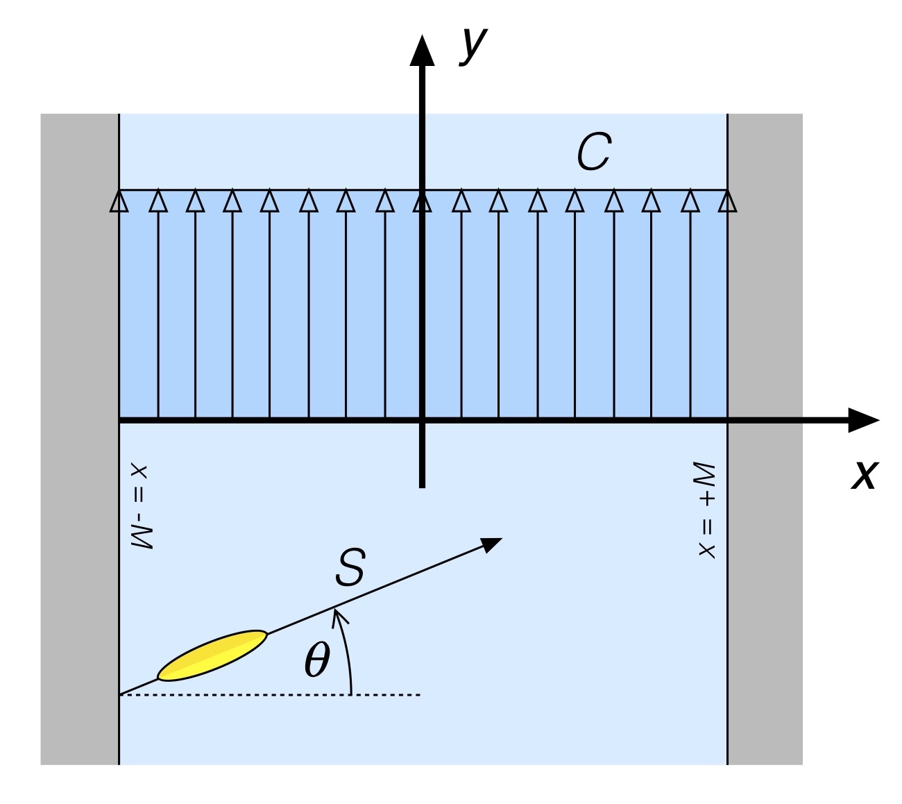
Fig. 1: River with uniform cross-stream current.

On the left bank a canoe is being paddled across the river at a constant speed S. In the absence of current the paddled hull’s keel line makes an angle $\theta$ with respect to the cross-stream (‘x’, or “spanwise”) direction.

Like in previous installments in the Science of Paddling series, we’re going to make a careful distinction between speed and velocity. Speed has magnitude only; it has no direction. For example, we could say that a car is going 100 km/hr because we read that number on our speedometer. That’s a speed; we often refer to quantities like this that have magnitude but no direction as scalars. Velocity has both magnitude and direction. It is an example of a vector. Driving 100 km/hr with a N/NE heading provides vector information.

Think of vectors like arrows. An arrow has a length (a scalar magnitude) and can be pointed in a direction. The canoe shown in Fig. 1 moves with a velocity vector shown as the labeled arrow. S represents the vector magnitude of the canoe’s velocity (e.g., its speed), while $\theta$ represents it direction in the absence of current. Vector notation often uses boldface (e.g., ‘S’) to more easily distinguish vector from scalar quantities (e.g., ‘S’) when you’re working your way through a page of math.

Vector quantities can also be written in terms of their component elements. These components comprise their projections along coordinate axes, like the x and y axes in Fig. 1. The canoe velocity vector S can be represented as an ordered pair of its scalar x and y components S_x and S_y as <S_x , S_y>, which are the portions of the canoe’s velocity in each coordinate direction, ordered by those direction so we know which piece is which. The angled brackets are just a common notation that lets us know this ordered pair of values is a vector, while the subscripts remind us which component part is which. In terms of the current-free hull angle $\theta$ , and using a little trigonometry, the vector S can be written as

$\mathbf{S}=\left\langle S\cos \theta ,S\sin \theta \right\rangle$

Similarly, the current is a vector since it has a magnitude C as well as a direction. It may not be a particularly interesting vector since it only has a single directional component, but it still has a direction, and we need to take this into account in our ensuing analysis. In Fig. 1 the current’s streamlines are aligned with the vertical (‘y’, or “streamwise”) axis, perpendicular to the spanwise direction. As a result, the current vector C, expressed in terms of its components, is

$\mathbf{C}=\left\langle 0,C \right\rangle$

Note that the current has no spanwise (‘x’) component.

Now recall that the angle $\theta$ represents the direction the canoe is being paddled in the absence of current. How can we determine its angle with respect to the river in the presence of current? Well, we use the beauty of vectors, and just add.

Fig. 2: Vector addition.

As shown in Fig. 2, vectors can be added pictorially by basically placing the “base” of one vector at the “tip” of another, making sure to preserve their respective angles, and measuring the resultant vector, the vector extending from the ”base” of the first vector to the “tip” of the second vector. That resultant vector is shown in the Figure as having magnitude R and direction $\phi$ . You can see that the current has turned the canoe’s direction of motion toward the flow direction. This does not mean that the canoe has rotated^[4]! Rather it means that the path describing the canoe’s motion – say, movement of the point corresponding to the hull’s center of rotation – is along the resultant vector R shown in Fig. 2, at an angle that is different than the angle defining the keel line.

Now we could do a little trigonometry to determine an expression for the resultant vector using the geometric construction shown in Fig. 2. But why work that hard? The beauty of representing vectors as ordered sets of scalar components like we did above lets us add vectors just using… addition. The resultant vector R is then derived from the canoe and current vectors as

$\mathbf{R}=\left\langle S\cos \theta ,S\sin \theta \right\rangle +\left\langle 0,C \right\rangle =\left\langle S\cos \theta ,C+S\sin \theta \right\rangle$

In vector addition you merely add respective scalar components – the x components of the vectors are added, and become the resultant vector’s x scalar component, and so forth – which is pretty sweet. No need to break out your trigonometry.

We now can determine how long it takes our canoe to cross the river in the presence of this current. We do this by calling upon high school physics, which taught us that distance is speed times time, and solve for time. Since we’re interested in determining how long it takes to cross the river, we only have to consider the x (e.g., cross-stream) component of the resultant velocity vector since that’s the direction of motion that gets us across. So using the cross-stream component of the resultant gives us

${{T}_{cross}}=\frac{2M}{S\cos \theta }$

There’s something nifty in this result: The time to cross the river has nothing to do with the current. It only has to do with the speed that you paddle the canoe in the absence of current, and the angle that you paddle it. Here, the angle is the angle of the hull’s keel line, not the angle of the resultant motion vector. Since the width of the river 2M is fixed, and we assume that you maintain a uniform speed S, the only variable is this angle of the hull with respect to the far shore.

What hull angle should you choose to minimize the time to cross the river? The one that maximizes the value of cos $\theta$ ; the larger the denominator, the smaller the fraction. Since the cosine function varies in magnitude from 0 to 1, the maximum value you can obtain for the denominator is S x 1. This occurs when… drum roll please… the angle $\theta$ equals 0, e.g. the canoe is pointed directly at the far shore. Another way of looking at this is that the crossing time is minimized when you put as much speed in the cross-stream direction as you can.

Now this probably isn’t surprising to most of you. You’ve paddled before. And you know that paddling this way you’ll get blown downstream, too! But keep in mind what question we were asking: How to minimize the time to cross the river for that type of current. In any optimization problem your result is determined by the stated goal. If you’re looking for minimum time to cross plus something else, that’s what we engineer’s call “feature creep.” It’s a different optimization problem.

A related question, knowing that the paddling speed S and river width 2M are fixed, is how do I choose the hull angle $\theta$ in order to minimize the distance traveled? Here’s where we can season our analysis with a liberal dose of common sense. The shortest distance between where you are on one shore to the far shore is… directly across. A straight line. Any other direction entails a longer path length (e.g., the magnitude R of the resultant direction of travel vector R) as you cross the river. So how do we choose the hull angle to minimize distance traveled in the presence of current?

With vector addition, of course.

Recall that the resultant vector R determined by the addition of the current-less canoe vector and the current vector has a component in the cross-stream direction, and a component in the downstream direction. If the component of velocity R in the downstream direction is zero then you won’t be blown downstream by the current. This is another way of saying that if you aren’t moving in a direction you won’t travel any distance in that direction, either. Using our ordered pair representation of R this means

$S\sin \theta =-C$

In other words, the canoe hull angle is set such that its downstream component (sin $\theta$ times S), e.g. its current-less downstream speed, exactly cancels the current’s magnitude. The reason you can see that it cancels is because of the minus sign. Basically, you’ve chosen a hull angle that transforms the vector addition into what’s depicted in Fig. 3. The current will push you downstream; with a precise choice of hull paddling angle you won’t be blown downstream but instead will travel directly across the river; you’re paddling upstream against the current. The resultant travel vector R is thus aligned with the cross-stream direction. Or in practice, close; the real world is a bit more dynamic, but you get the idea.

Fig. 3: Minimum distance crossing resultant in uniform cross-stream current.

And what if the current’s magnitude C is greater than your paddling speed S? First, the minimum distance solution goes out the window. You can see this by letting the current magnitude be greater than the paddling speed S by an amount $\Delta$ . Then you can never satisfy the equation above, since

$S\sin \theta =-C\to S\sin \theta =-(S+\Delta )n$

Dividing by S and taking the magnitude of both sides of this equation shows that you would have to find a hull paddling angle that satisfies

$\left| \sin \theta \right|=\left| 1+{}^{\Delta }\!\!\diagup\!\!{}_{S}\; \right|$

There is no angle $\theta$ that makes this possible for any value of $\Delta$ greater than 0 because the magnitude of sin $\theta$ can never be greater than 1. You just don’t have enough oomph to paddle straight across when the current is that strong!

Another obvious case is when you decide to call it a day, turn the boat downstream, and head for a takeout on the same side of the river as you start from. One way of representing this case is by choose a current-free hull paddling angle $\theta$ equal to 90 degrees. Then,

${{T}_{cross}}=\frac{2M}{S\cos \theta }\to \frac{2M}{S\cos \left( 90\text{degrees} \right)}=\frac{2M}{0}\to \infty$

Your river crossing time becomes infinite because you never cross the river! Obvious, yeah. But when infinities pop up in any analysis they are usually trying to tell you something; either the math’s wrong, the problem isn’t well posed, or the infinity needs to be interpreted in terms of reality. As to whether it would actually take an infinite amount of time, well, who’s got that much free time to check?

EXTENSION TO OTHER CURRENT PROFILES

A current having a uniform cross-stream profile may occur in canals, and can be a reasonable first approximation for a number of rivers. But what about crossing a river in a bend, where the current often piles up along the outer shoreline? Or a river with variable cross-stream depth, say one deepest in the middle but shallow along the banks? Can the analysis above be generalized? Without (fingers crossed) using variational calculus?

Well, sure; we can approach these with somewhat more general current profiles. And appeal to our intuition now that we’ve gotten the uniform current profile case under our belts. We’ll start first by unbending a river.

So how do you unbend a river? Well, if the river has a bend where the current increases (say) linearly from the inner shoreline to the outer, we can imagine taking a cross-stream slice of the river along a radius, and say that we’ve got a slice that for at least a little distance upstream and downstream looks like a piece of a straight river having the current profile shown in Fig. 4.

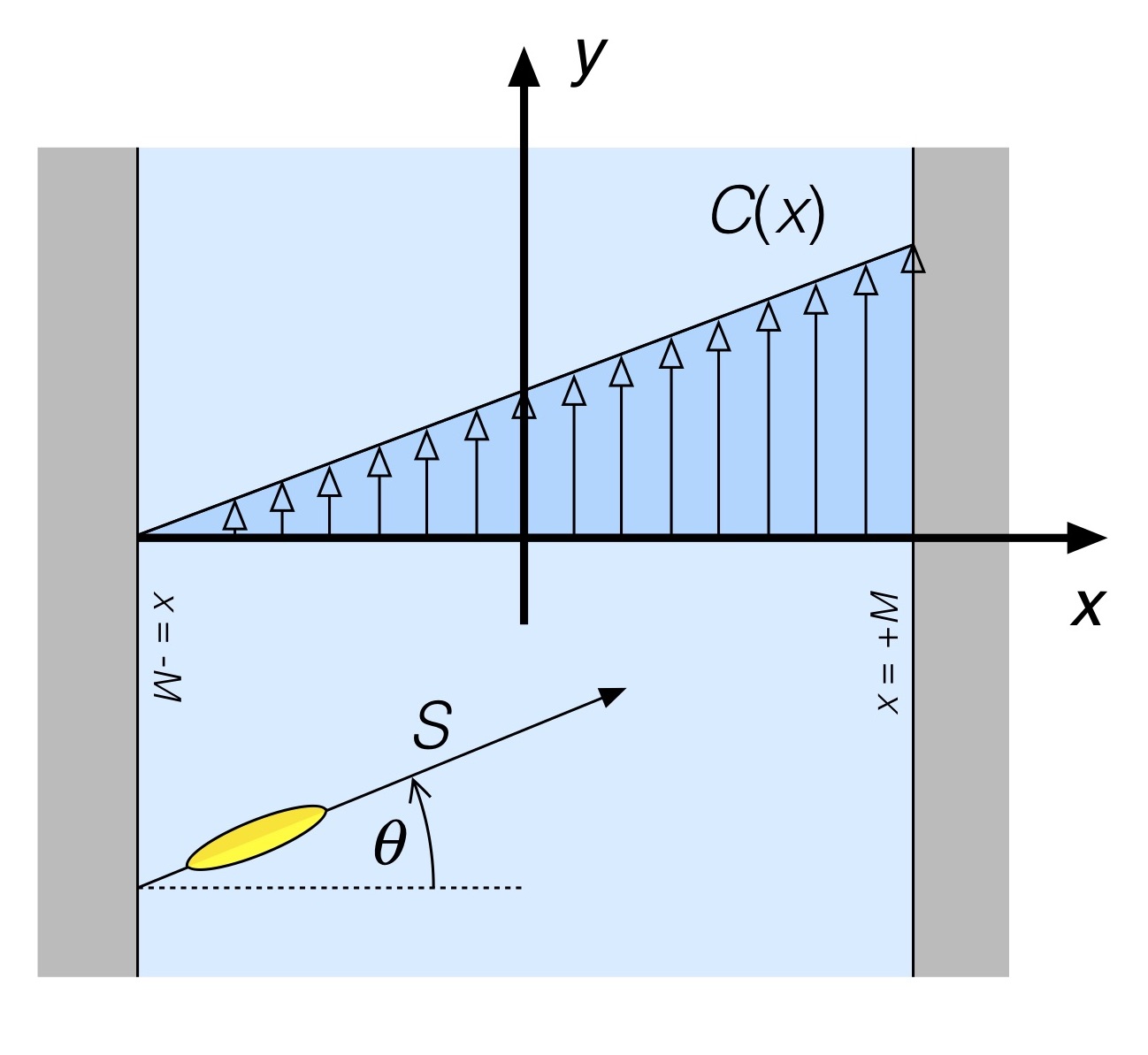
Fig. 4: River with linear cross-stream current profile.

If the river is really twisty you’ll need to solve the problem in polar coordinates, but for a more gradual turn this is a reasonable approximation.^[5] At first blush this doesn’t look all that much like the uniform cross-stream current case. But if we introduce another approximation (which we’ll later dispense with), it does. Let’s approximate the current profile of Fig. 4 by assuming that over successive “chunks” of the cross-stream direction the current doesn’t change all that much. One such approximation is shown in Fig. 5.

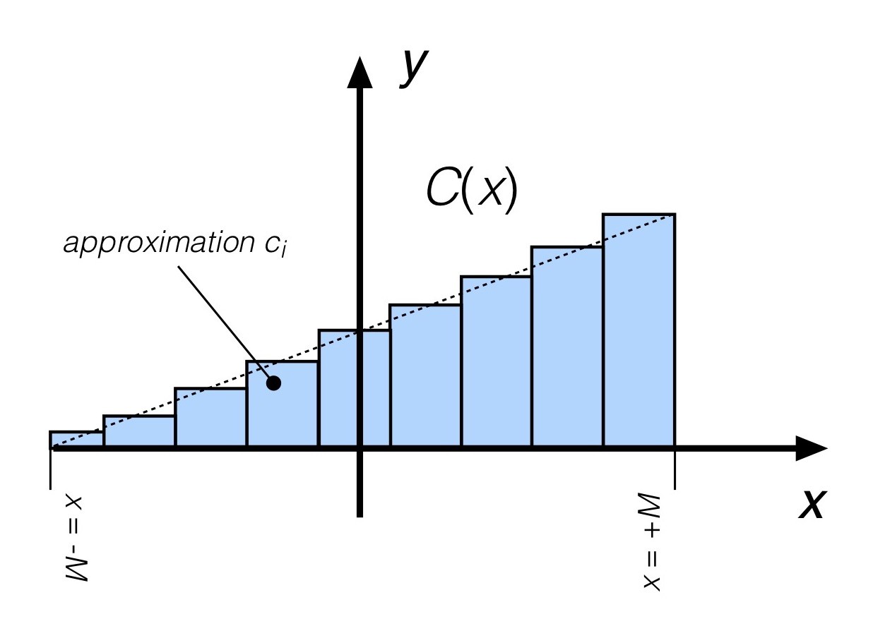
Fig. 5: Stepwise approximation of the linear cross-stream current profile.

Here, the current is assumed to be uniform over each of a number of adjoining steps. The current magnitude in each is merely the value of the actual current C at (say) the center of each step. This is an example of a stepwise approximation of the function C(x), something that will be familiar to anyone who has done numerical integration or digital signal processing.

Let’s assume that the current magnitude in the i^th step is represented by the scalar c_i. Consider first the first segment, e.g. the one adjoining the side of the river you are paddling from. In this first segment you now have the uniform spanwise current case we examined previously (!) for a somewhat narrower “river” (e.g., the channel corresponding to this first step across the river), now for a local current value c₁. And we already know how to minimize the crossing distance in that case: choose a hull paddling angle to counteract the current. For this first segment,

${{\mathbf{R}}_{1}}=\left\langle S\cos \theta ,S\sin \theta \right\rangle +\left\langle 0,{{c}_{1}} \right\rangle =\left\langle S\cos \theta ,{{c}_{1}}+S\sin \theta \right\rangle$

As before, to prevent drifting downstream over the first segment we need to null out the resultant velocity in the downstream (‘y’) direction. Which means

$S\sin \theta =-{{c}_{1}}$

Using a little trigonometry, you can determine the angle $\theta$ via

$\theta =\arcsin \left( -{}^{{{c}_{1}}}\!\!\diagup\!\!{}_{S}\; \right)$

As for the 2^nd step in the current approximation, as long as the current isn’t strong enough over the segment to blow you downstream you’d do the same thing; you already crossed the first segment optimally with no downstream drift, and are still heading straight across the river when you start the 2^nd step. As you have probably already deduced, you can repeat this process across all steps. Nulling the resultant downstream velocity over each step means satisfying

$S\sin \theta =-{{c}_{i}}$

Which leads to a current-free hull angle over each segment of

$\theta =\arcsin \left( -{}^{{{c}_{i}}}\!\!\diagup\!\!{}_{S}\; \right)$

Since here the current magnitude c_i in any segment will differ from that in other segments, the hull angle in each will consequently be different. You’ll be constantly adjusting your hull angle in each segment.

You may have noticed that the analysis in this section hasn’t assumed how many steps are used to approximate the linear cross-stream current variation. Which means you could use as many as you’d like. Like, say a lot. A whole lot. The more you use, the better the approximation of the actual current profile. And in each we have a way to adjust hull angle to keep you heading straight across the river. As the segments get narrower and narrower you start to approach a continuum of values. In calculus this argument is often referred to as “taking the limit” where either something goes to zero (like the step widths here), or to infinity. In the limit here at any spanwise location x, your current-free hull paddling angle would then have to satisfy

$S\sin \theta =-C\left( x \right)$

Which leads to the angle being expressed as

$\theta =\arcsin \left( -{}^{C\left( x \right)}\!\!\diagup\!\!{}_{S}\; \right)$

The angle $\theta$ is now continuously varying since the argument of the arcsin function varies with position across the river. Note also that the angle depends on the ratio of the current C and the hull speed S, not on their individual values. And it does not depend on the river’s width.

So what does this angular variation look like? Pretty much what you’d expect, as seen in Fig. 6.

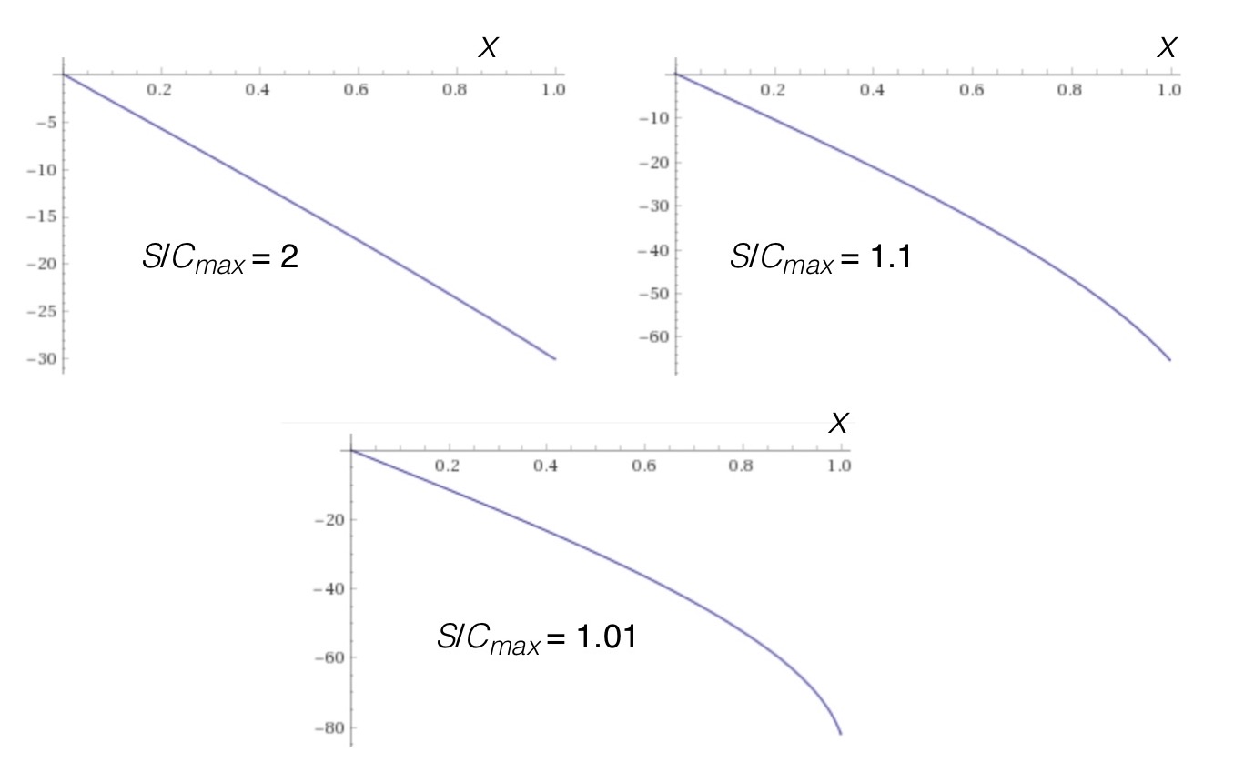
Fig. 6: Hull angle vs. distance for various ratios of hull speed and maximum current speed for the linear current profile.

In each plot of Fig. 6 the river has been “shifted” and scaled to have width 2M = 1, with the cross-stream coordinate extending from the left bank (x = 0) to the right bank (x = 1); this is just a convenience for computation and plotting. The three cases correspond to ratios of hull speed to maximum current of 2 (hull speed twice as fast as the current), 1.1 (hull speed 10% faster than the current), and 1.01 (hull speed only 1% faster than the current). In all three cases the hull speed is much faster than the current on the left side of the river, so the current-free hull angle scarcely varies until you paddle beyond mid-stream. With increasing current magnitude as you approach the far shore the canoe has to be turned progressively more into the current so as to continue straight across. In the case where the hull speed is scarcely larger than the maximum current magnitude for this case, the hull is pretty much running parallel to shore to work against the current and not be swept downstream. Bottom line: For hull speeds much greater than the maximum current magnitude, for this current profile you can pretty much ignore the current variation, set your angle, and paddle across with minimum distance. For this current profile you only need to introduce cross-stream hull angle changes when the maximum current is strong, and that changes progressively as you enter stronger and stronger current.

And what about the time to cross for this linear cross-stream current profile? Will the changing current alter our “paddle straight across” approach for minimizing time?

Short answer: No. The resultant velocity vector for any cross-stream variation in current magnitude C(x) takes the form

$\mathbf{R}=\left\langle S\cos \theta ,S\sin \theta \right\rangle +\left\langle 0,C\left( x \right) \right\rangle =\left\langle S\cos \theta ,C\left( x \right)+S\sin \theta \right\rangle$

Recall that the time to cross only depended on the cross-stream component of the resultant. And for any variable current profile with parallel streamlines that are aligned with the riverbank, the current does not contribute any “push” across the river, just along it^[6]. So consistent with these assumptions, to minimize the time to cross the river, always paddle straight across.

As a last example we’ll consider a river having variable depth, with symmetric cross-stream bathymetry, having a parabolic cross-stream current profile. This is depicted in Fig. 7.

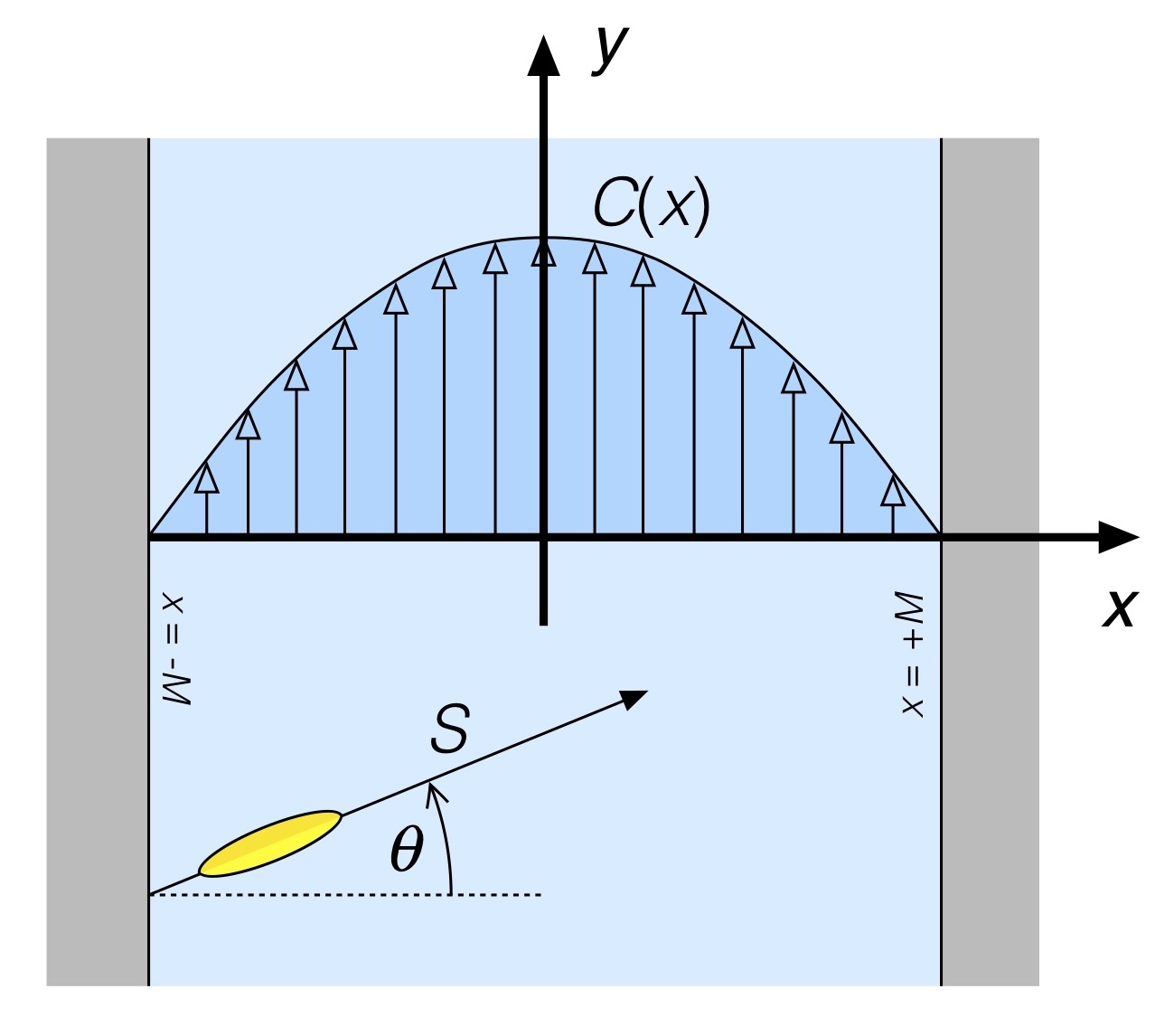
Fig. 7: River with parabolic cross-stream current profile.

By now you know the drill. The current profile can be approximated by a series of discrete “sub channels” of the river, each assumed to have constant spanwise current magnitude with value equal to the magnitude of C(x) at its center. The analysis proceeds as before, taking more and more, and finer and finer discretizations until the continuous current profile is recovered. We already know that the minimum time solution means paddling straight across since the streamlines are all parallel to the major axis of the river. It’s just that the current-free hull paddling angle will now vary across the river with even symmetry about mid-stream, as shown in Fig 8.

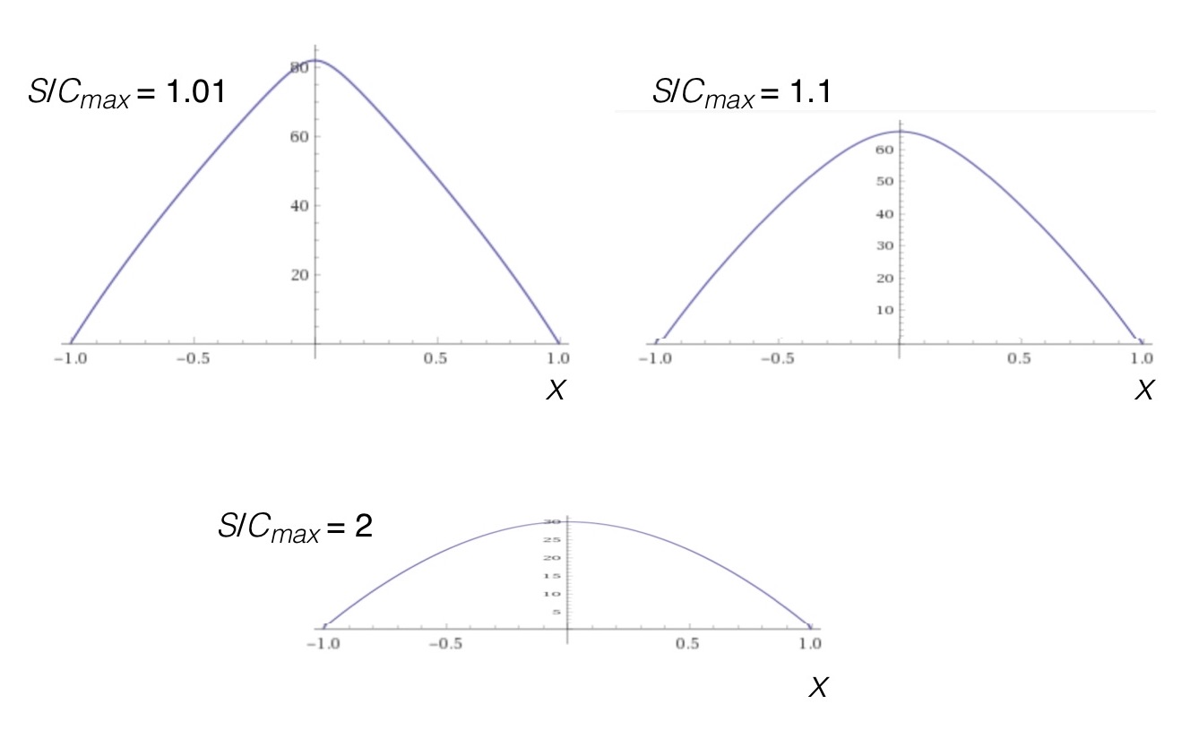
Fig. 8: Magnitude of hull angle vs. distance for various ratios of hull speed and maximum current speed for the parabolic current profile.

In each plot of Fig. 8 the river has been “shifted” and scaled to have width M = 2, with the cross-stream coordinate extending from the left bank (x = -1) to the right bank (x = 1); this is just a convenience for computation and plotting. The three cases correspond to ratios of hull speed to maximum current of 2 (hull speed twice as fast as the current), 1.1 (hull speed 10% faster than the current), and 1.01 (hull speed only 1% faster than the current). In all three cases the hull speed is much faster than the current near the shorelines, so the current-free hull angle is zero as you begin and conclude your crossing. With increasing current magnitude as you approach midstream the canoe has to be turned progressively more into the current so as to continue straight across; note that while the curves all look similar, the maximum angles on the abscissas of the plots differ in each case. In the case where the hull speed is scarcely larger than the maximum current magnitude, at mid-stream the hull is nearly running upstream to work against the current and not be swept downstream. And in each case the hull angle varies the most when you’re furthest from shore, not doubt making it harder to decide what angle to set since on the water you’d have to be watching both the far shore (to your left) and the orientation of the keel line (straight in front of you). A bit more to manage. But it can be done.

CONCLUSION

In this installation of the Science of Paddling series we’ve considered two optimization problems: How to cross a river in minimum time, and in minimum distance. For rivers having parallel streamlines with no cross-stream component the shortest time to cross always entails paddling straight across. And for the minimum distance problem, well, you want to travel straight across; you just need to adjust your hull angle while doing so to “cancel out” any current effects. And we did it by drawing pictures, and doing addition. Not bad for a day’s work. The minimum distance analysis here is at least locally optimal, in that the solution is optimal point-by-point for each location across the river. I have to verify whether or not it is globally optimal (which would consider the entirety of the current profile in computing the requisite hull angles rather than just the local value of the current. This will be relevant in subsequent articles outlined below.)

This type of analysis can be extended quite easily to the problem of starting at one location on the near shore and trying to hit a location on the far shore with minimum (straight line) distance. Just determine the bearing to your target location and use vector addition to solve for the hull paddling angle which provides a resultant velocity vector pointing along the target bearing. The proof, as they say, is left to the reader.

Perhaps a more interesting problem is that of determining the path resulting in a minimum time to cross going from an upstream location to a downstream location. This problem is more akin to downstream racing than hopping eddies. Let’s save it for the sequel, “Even More Rivers to Cross.”

And finally, a problem of particular interest to me is that of crossing a river with minimum energy expenditure. This is of interest to marathon racers, for example. I started sketching out the solution but realized that this article was long enough already. And I’d like to minimize my energy expenditure for today.

v1.0

And I have often wondered, “How do I get across without going for a long, cold swim?” But that’s an article for another time… ↑
I know some of you will be disappointed. ↑
Which is a nice way of saying, “I know the answer, and it was cleaner to derive using this way of representing the width.” ↑
Although poking your nose across an eddy line will rotate the hull; here we’re considering the idealized case of no differential currents. ↑
Or at least as good an approximation as assuming a linear spanwise current profile! ↑
Real rivers have currents that go all over the place. It’s just challenging to come up with a representative model for spanwise current that applies to a number of rivers rather than a few isolated cases. And without introducing more math. ↑

The Science of Paddling

The intersection of physics, physiology, and paddle sport

Category Archives: Mathematics

Part 18: Many Rivers to Cross