
by Shawn Burke, Ph.D.
OVERVIEW
The Global Position System (GPS) is summarized, including an overview of how trilateration is used to determine a receiver’s location. A brief history of mobile GPS systems for sport and consumer products of the late 1990s and early 2000s is presented.
INTRODUCTION
A few key technological innovations during the 1980s and 1990s led to the development and commercial introduction of mobile devices with integral Global Positioning System (GPS) receivers. The enabling innovations included the availability – and opening to civilians – of the GPS system, as well as advances in the miniaturization of energy efficient computer processors.
The Global Positioning System (GPS) is a satellite-based navigation system that was developed by the U.S. Department of Defense in the early 1970s. The GPS system consists of a “constellation” of 24 satellites in circular orbits above the Earth, distributed such that 4 to 10 satellites are visible anywhere in the world at any time. Each GPS satellite transmits a radio frequency (RF) signal. The signal is comprised of two carrier frequencies upon which are modulated digital codes, plus a navigation message. A receiver uses the transmitted carriers and codes to determine the distance (aka, range) from it to the GPS satellites, as described below. The system is depicted conceptually in Fig 1.
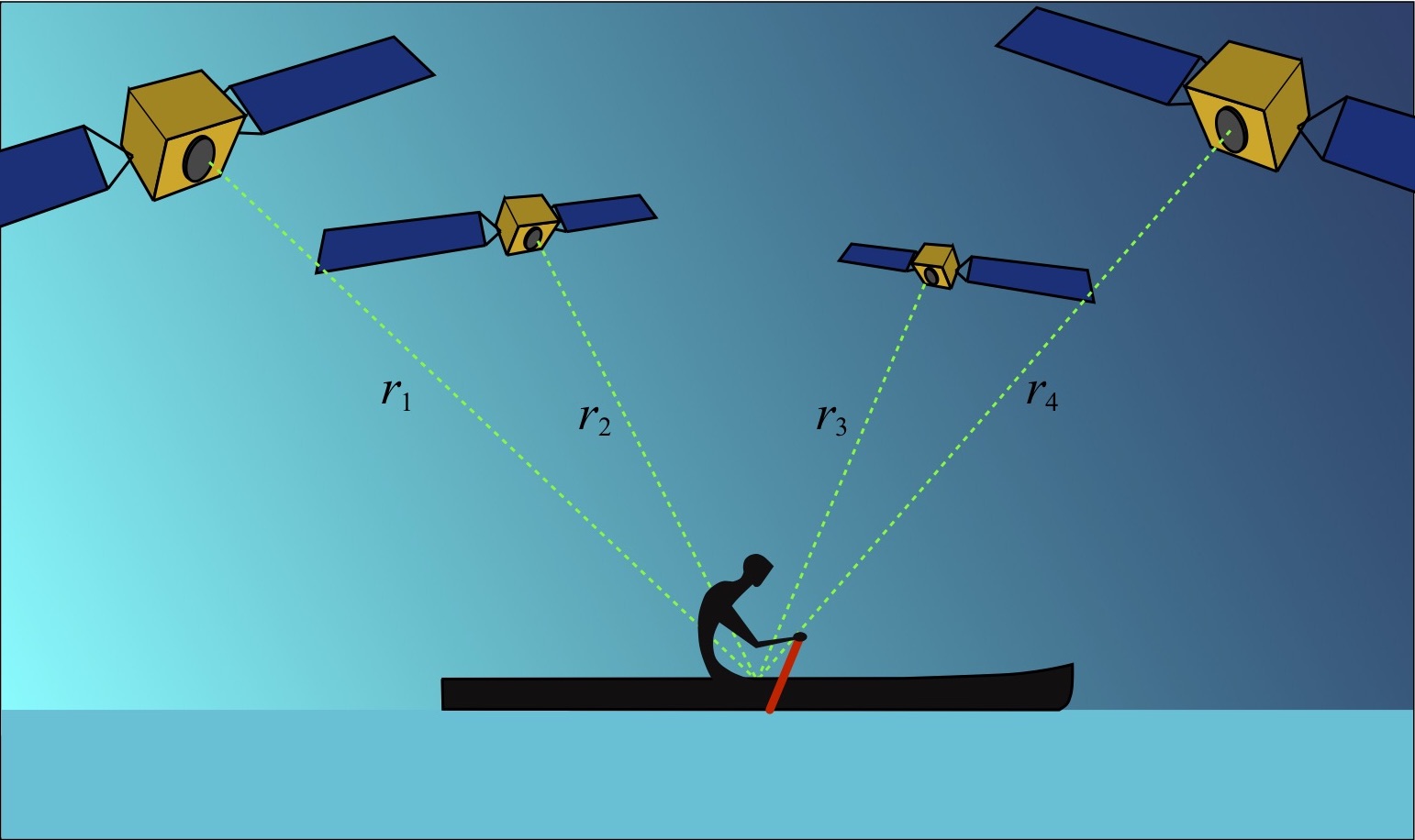
Figure 1: GPS satellites, and receiver aboard a C-1 for determining ranges and position.
HOW THEY DO IT
In order to determine your location using GPS, your GPS receiver performs a number of steps. It first receives a radio frequency (RF) signal from each of at least four GPS satellites. It determines the range to each of these. Then it performs a series of mathematical operations to determine your location and velocity.
Your GPS receiver determines the distance to a GPS satellite by measuring the time it took the RF signal transmitted from the satellite to arrive. The process for accomplishing this unfolds as follows[1]. At a pre-determined start time a satellite begins to transmit a long digitally encoded message called a pseudo random code. Examples of the waveforms corresponding to these codes are shown in Fig. 2.
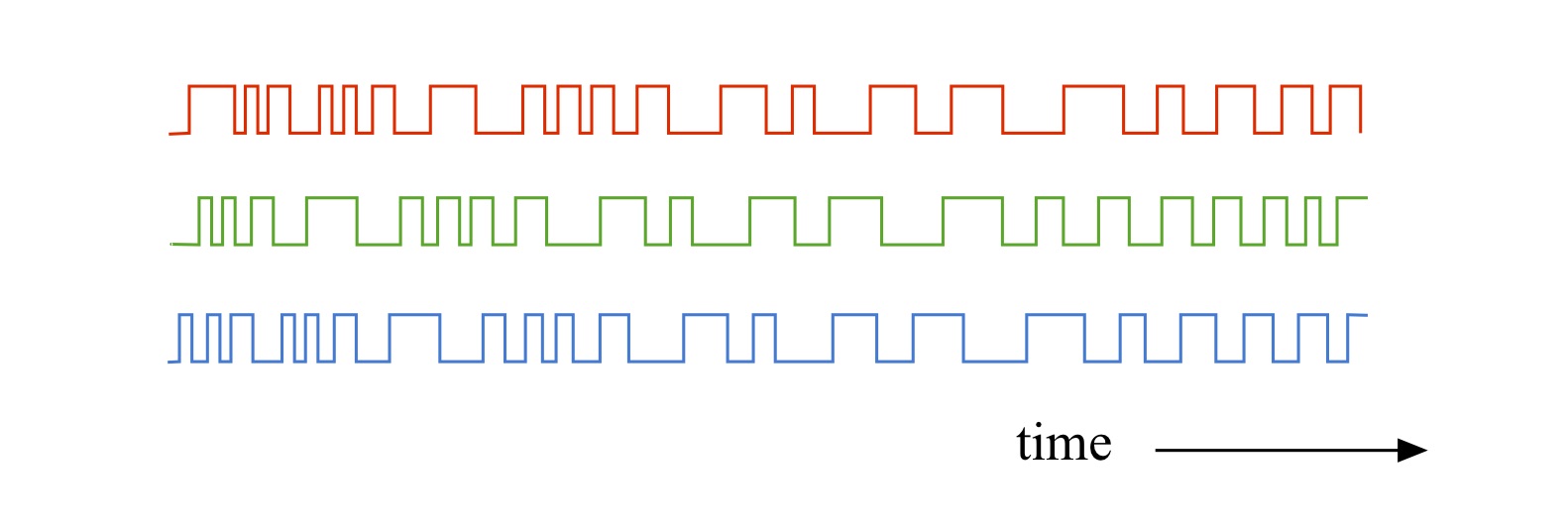
Fig. 2: Examples of pseudo random code waveforms from three different satellites.
At the same start time the receiver also generates its own copy of this encoded message, but does not transmit it. The corresponding reference code waveform generated by the receiver is then compared to the coded waveform received from the GPS satellite, as suggested in Fig. 3.
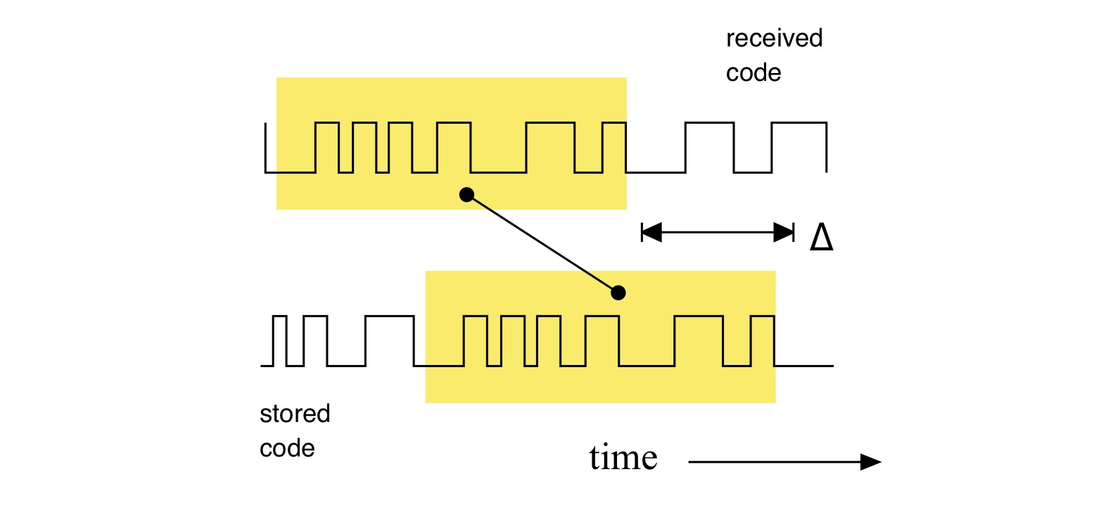
Fig. 3: Time lag between reference and received pseudo random codes.
As shown in the figure matching segments of the two waveforms – one from the satellite, the other generated by the receiver – are identified, and their relative timing is determined. The received waveform lags the reference waveform by an amount of time ∆. This is because it takes a finite amount of time for the RF signal to propagate from the satellite to the receiver even though the signal travels at the speed of light. Multiplying this time lag by the speed of light yields the distance (e.g., range) to that satellite. Adjustments are made to account for atmospheric phenomena that influence the signal transit time.
The signal from the GPS satellite also includes a navigation message. The navigation message comprises the coordinates of the satellite as a function of time, as well as information used to correct the range measurements derived by a receiver that account for atmospheric phenomena which influence the signal transit time as noted above. The received waveform also includes address information that allows the receiver to determine which GPS satellite transmitted the pseudo random code waveform.
The satellites travel in precisely known orbits. So knowing the 3D position of one satellite (x1,y1,z1) and its range r1 to the receiver means that the receiver knows that its own location lies somewhere on the surface of a sphere of radius r1 centered at the location of the satellite. This is illustrated in Fig. 4(a). Merely knowing the range to one satellite is not enough information for the receiver to determine its own 3D location. In order to do this the receiver performs trilateration, a 3D version of triangulation.
Modern GPS receivers can determine the range to multiple GPS satellites at one time. Trilateration involves combining position and range information from these multiple satellites, as shown in Figs. 4(a) through 4(c).
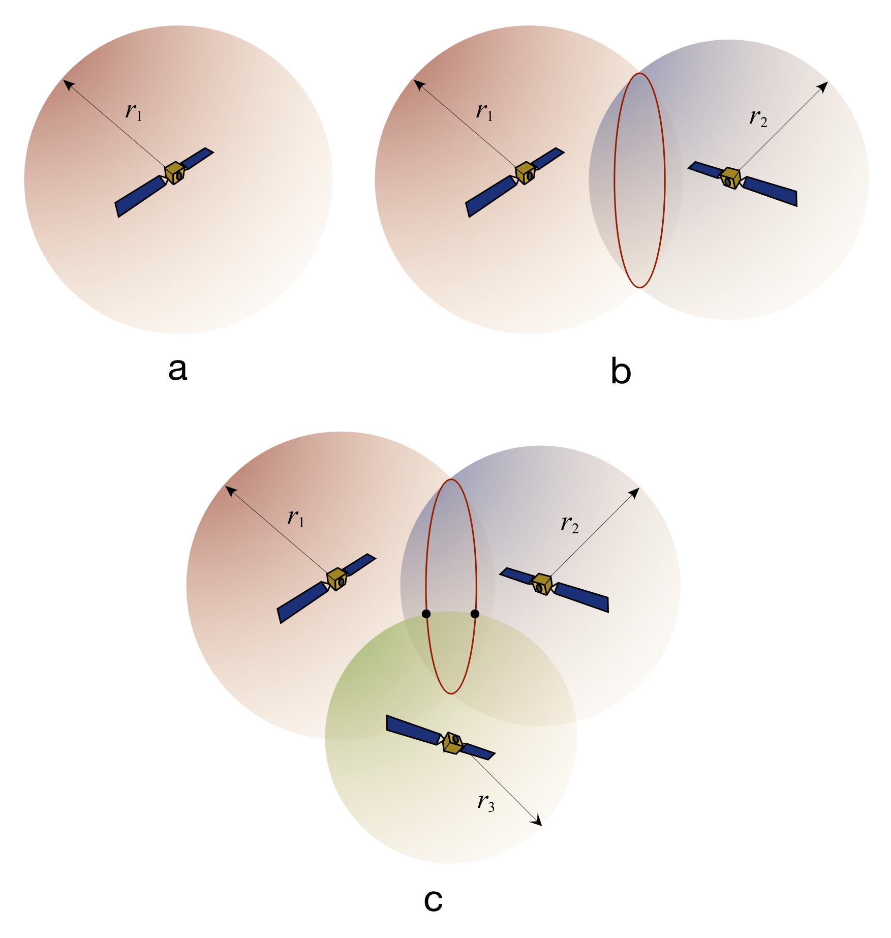
Fig. 4: Trilateration steps.
Trilateration works as follows. First, the location of and range to a first satellite constrains the receiver’s location to being somewhere on a sphere, as shown in Fig. 4(a). Combining this with the position of and range to a second satellite means that the receiver position must lie somewhere along the intersecting ring of two satellite “range spheres” as shown in Fig. 4(b), since (in general) spheres intersect along a 2D ring. Adding a third satellite’s position and range information means that the GPS receiver’s location must be at one of two points corresponding to the intersection of the third satellite’s “range sphere” and the aforementioned intersecting ring, as shown in Fig. 4(c). This means the receiver must be located at one of the two dots shown in Fig. 4(c). And finally, since the receiver is constrained to lie somewhere on (or in the case of aviation receivers, near) the surface of the Earth, the GPS receiver’s location must be at the proximate intersection point as shown in Fig. 5. Congratulations! You’ve just located yourself in 3D space using signals from three GPS satellites.
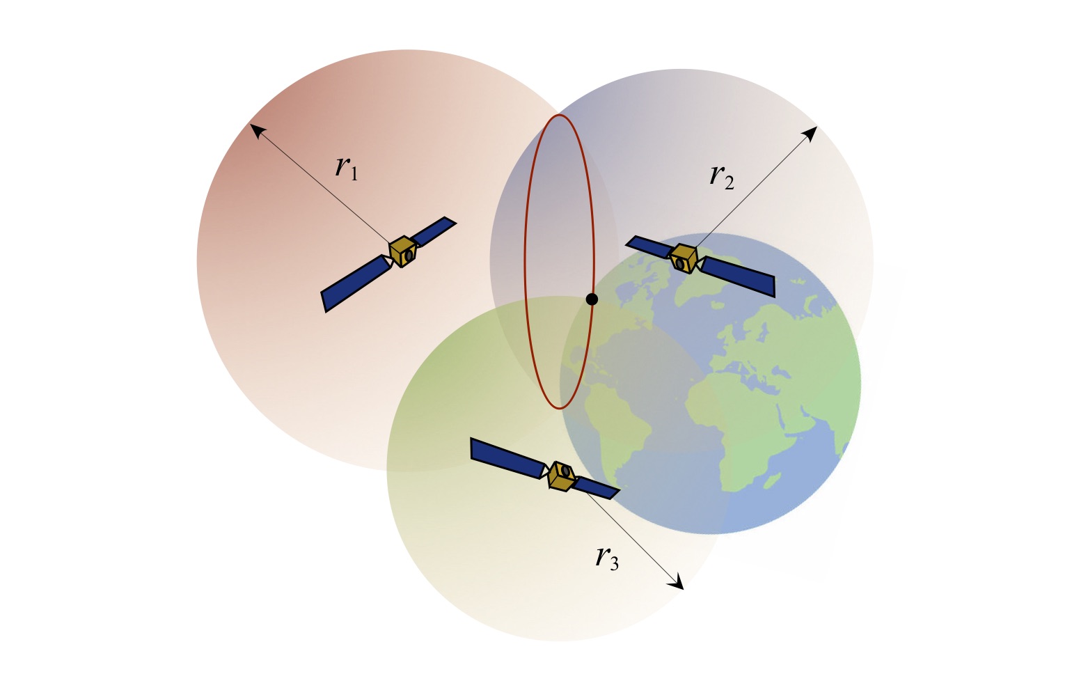
Fig. 5: Final trilateration step.
In order to obtain an accurate position estimate trilateration requires the clocks in both the satellite and the receiver to be synchronized. The satellites themselves have atomic clocks, extraordinarily accurate[2] time and frequency references. The receivers have more conventional quartz crystal-referenced clocks that drift – e.g., run fast or slow – in comparison. This drift of the receiver’s clock with respect to the GPS satellites’ clocks means that the range computations will be slightly off. We’ll write the drift in the receiver clock time as 
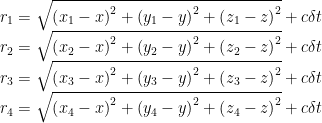
In these equations c is the speed of light, so that the term c
And what about velocity? The obvious way to calculate the receiver’s velocity is to take the difference between two successive position estimates, subtract, and divide by the time between these two measurements. For example, if a hull is traveling at 6.7 mph (3 m/s), and the sampling period between position measurements is 6 sec, over that time you’ve traveled 18 meters. But each GSP position estimate has an error associated with it.
Prior to May 2, 2000, GPS accuracy for civilian receivers was approximately 100m for horizontal position and 156m for elevation. This is because GPS signals were intentionally degraded for security reasons. This degradation – known as “Selective Availability” – was removed by the United States government on May 2, 2000, resulting in an accuracy improvement of a factor of seven or more.
If the error in each position estimate is (for example) 5 meters, then your computed velocity could be 3 m/s if these two errors perfectly cancel each other – recall that velocity is a vector. Or, 18 meters actually traveled plus two times 5 meters (one possible worst-case error) leads to an overly optimistic 4.67 m/s (10.45 mph). Or 18 meters actually traveled minus two times 5 meters (another possible worst-case error) leads to a woefully pessimistic 1.33 m/s (3 mph). Yipes!
An example of position errors from a trail run in the local Deer Jump Reservation is shown in Fig. 6. The various waypoints along this out-and-back route are connected with red lines. The trail itself is at most 2m wide over much of its length. But owing to a variety of factors what “should” be almost perfectly overlaid traces is instead a pair of meandering tracks that sometimes intersect, but often don’t.
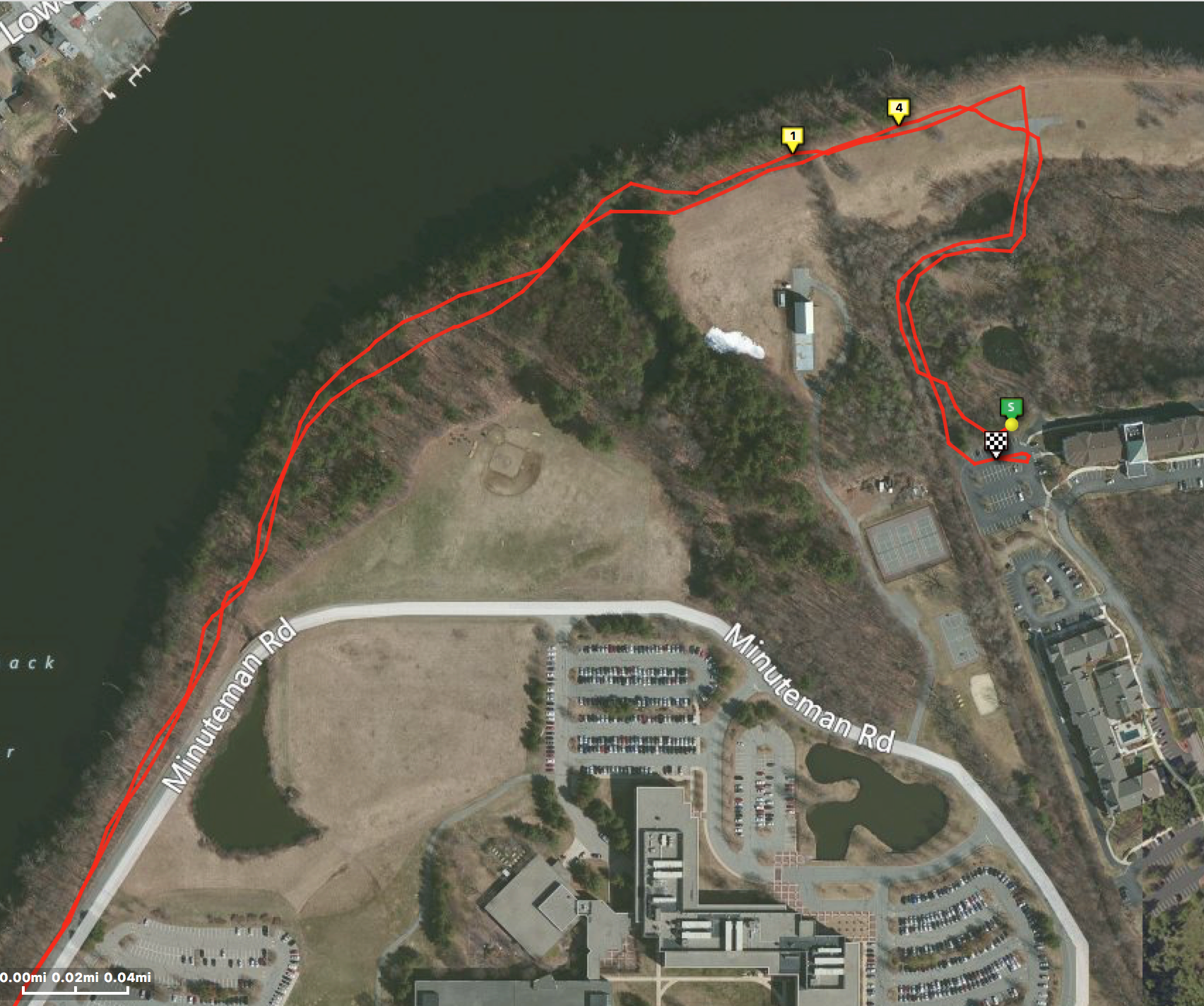
Fig. 6: GPS waypoints from an out-and-back trail run.
Another limitation of the “subtract and divide” approach for computing velocity is that this estimate is not instantaneous. It relies on a present data point, plus a data point obtained some amount of time in the past. So even if it were accurate it would represent some average velocity in the past, rather than your present instantaneous velocity. Over the span of an entire workout or race it’s probably okay to use the total distance divided by the total time to compute average speed since the errors associated with each position estimate will (hopefully) be uncorrelated. But using this approach to compute instantaneous speed is fraught.
Instead, GPS receivers use the Doppler shift of the signal it receives from a satellite to compute velocity.[4] You’ve heard a Doppler shifted acoustic signal if you’ve ever listened to a train horn as the train recedes into the distance. The relative velocity between you and the train causes the apparent speed of sound between you and the horn to change as the train passes. Consequently, the tone you hear from the train horn drops in frequency as it passes. In a similar way, your movement with respect to the GPS satellite causes a shift in the frequency of the radio signal acquired by your receiver. Also, the satellite has an approximately 7 km/sec orbital velocity; it’s moving, too. And the Earth has a rotational velocity that ranges as high as 400 m/sec at the equator. Taking all of these into account allows a GPS receiver to compute your instantaneous velocity.
EARLY MOBILE GPS FOR SPORTS
The price and availability of commercial GPS receivers changed radically between 1980 and 2002. As Ahmed El-Rabbany noted in 2002[5]:
In 1980, only one commercial GPS receiver was available on the market, at a price of several hundred thousand U.S. dollars. This, however, has changed considerably, as more than 500 different GPS receivers from more than 70 companies are available in today’s market… The current receiver price varies from about $100 for the simple handheld units to about $15,000 for the sophisticated geodetic-grade units. The price will continue to decline in the future as the receiver technology becomes more advanced.
GPS receivers became widely available for outdoor applications such as hiking, boating, and vehicle navigation. By the mid-1990s, companies such as Garmin, Trimble, and Magellan offered a variety of hand-held GPS devices to consumers; I personally owned and used a Garmin GPS II Plus in 1998, and first used it paddling during a backcountry trip in Temagami. I still have it, although the battery-backed static ram (SRAM) memory no longer functions (and the manufacturer no longer services this model); the GPS II Plus was built before flash memory became common.
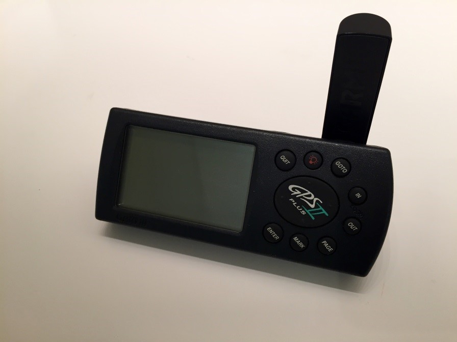
Figure 7: Garmin GPS II Plus
In 1997 a team of MIT students built and publicly demonstrated a wearable system referred to as “Marathon Man” that sensed a runner’s heart rate, step cadence, core body temperature, and GPS position, used the GPS information to determine the runners’ speed; and periodically transmitted that information via a cellular phone or cellular modem to a remote internet-connected control center, while the runners were still traversing the course.[6] At the control center runner position and physiological status was graphically displayed and updated throughout the race. The Marathon Man system was used successfully during the 1997 San Francisco Marathon, as documented in a September 1997 broadcast of the ABC Nightly News.[7]
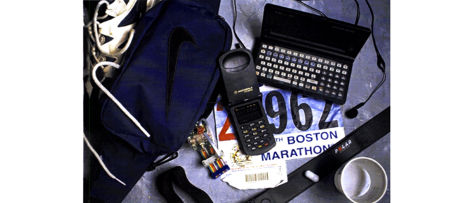
Figure 8: Marathon Man” system components (source: Redin MS Thesis, pp. 2).
In 2000, Garmin introduced the eTrex Summit handheld GPS “Personal Navigator.” The eTrex Summit displayed a user’s animated location on a map, elevation and elevation change over time or distance, total ascent and descent, recorded and labeled waypoints, determined speed / average speed / maximum speed, enabled the creation and following of routes including routes uploaded from a PC, and could record a “track log” of time-stamped waypoints including elevation data. A waypoint is simply a location along a route. A waypoint position could be entered by taking a GPS fix, by manually entering coordinates, or by referencing a bearing and distance to a known position.
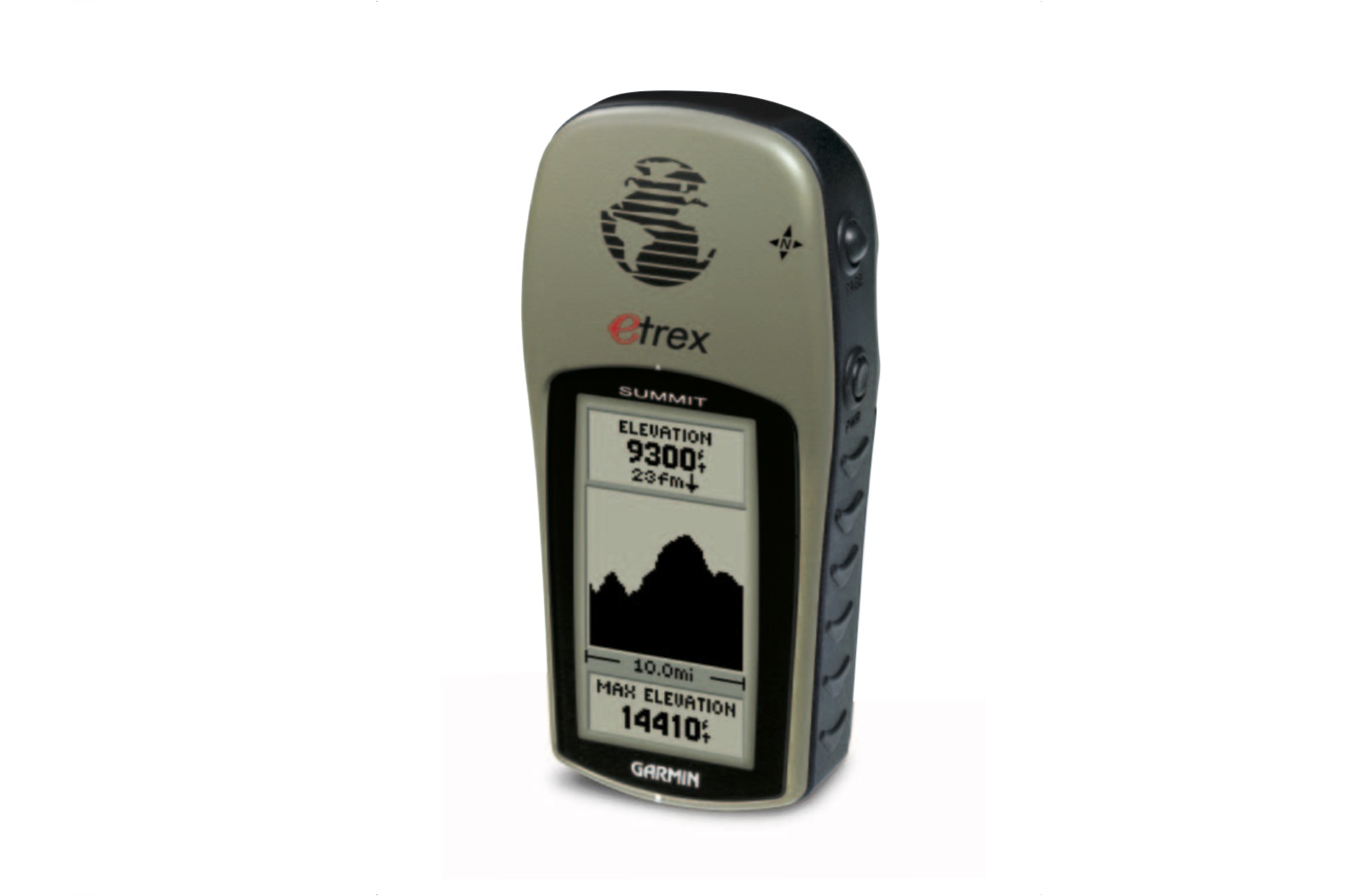
Fig. 9: Garmin eTrex Summit (source: eTrex Summit Owner’s Manual and Reference Guide).
Starting in 2001 GPS receivers were integrated into handheld Personal Digital Assistants (PDAs). For example, in 2001 Geode introduced the GPS Springboard Module for the Springboard PDA. The Geode was a plug-in GPS module for the Handspring Visor PDA. It combined a GPS receiver, Web-based travel content, and mapping software that turned the Handspring Visor into an electronic travel guide. Devices combining GPS with a cellular phone started appearing in 1999. The Benefon Esc (publicly introduced in 1999 and first sold in 2001), the Garmin NavTalk (first sold in 1999) and the Garmin NavTalk GSM (first sold in 2003) combined GPS and cellular communications technology. The Benefon Esc and the NavTalk GSM were also capable of transmitting and receiving position and speed information over wireless networks. The Esc had an optional bracket mount for cycling, and could also send and receive data sets corresponding to entire routes.
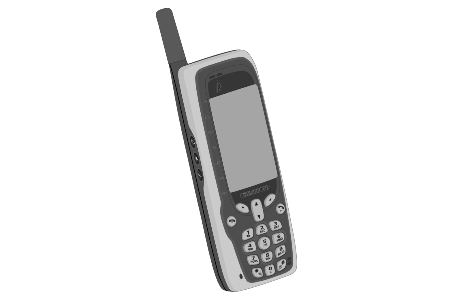
Figure 10: Benefon Esc (2002 model).
In 2004 Timex introduced the BodyLink fitness sensor system. The BodyLink comprised four distinct parts that were wirelessly linked: a sports watch for receiving and displaying data, a wireless heart rate sensing chest strap, a GPS receiver, and a data recorder, as shown in Fig. 11. The GPS receiver was not integrated into the watch. It was designed to be worn on the shoulder of your shirt or singlet, or attached to your belt; I strapped mine to a thwart. The separate data recorder was required if you wanted to download data from your workout for later analysis. The receiver in the BodyLink model I owned was manufactured by NavMan, and Australia / New Zealand company.
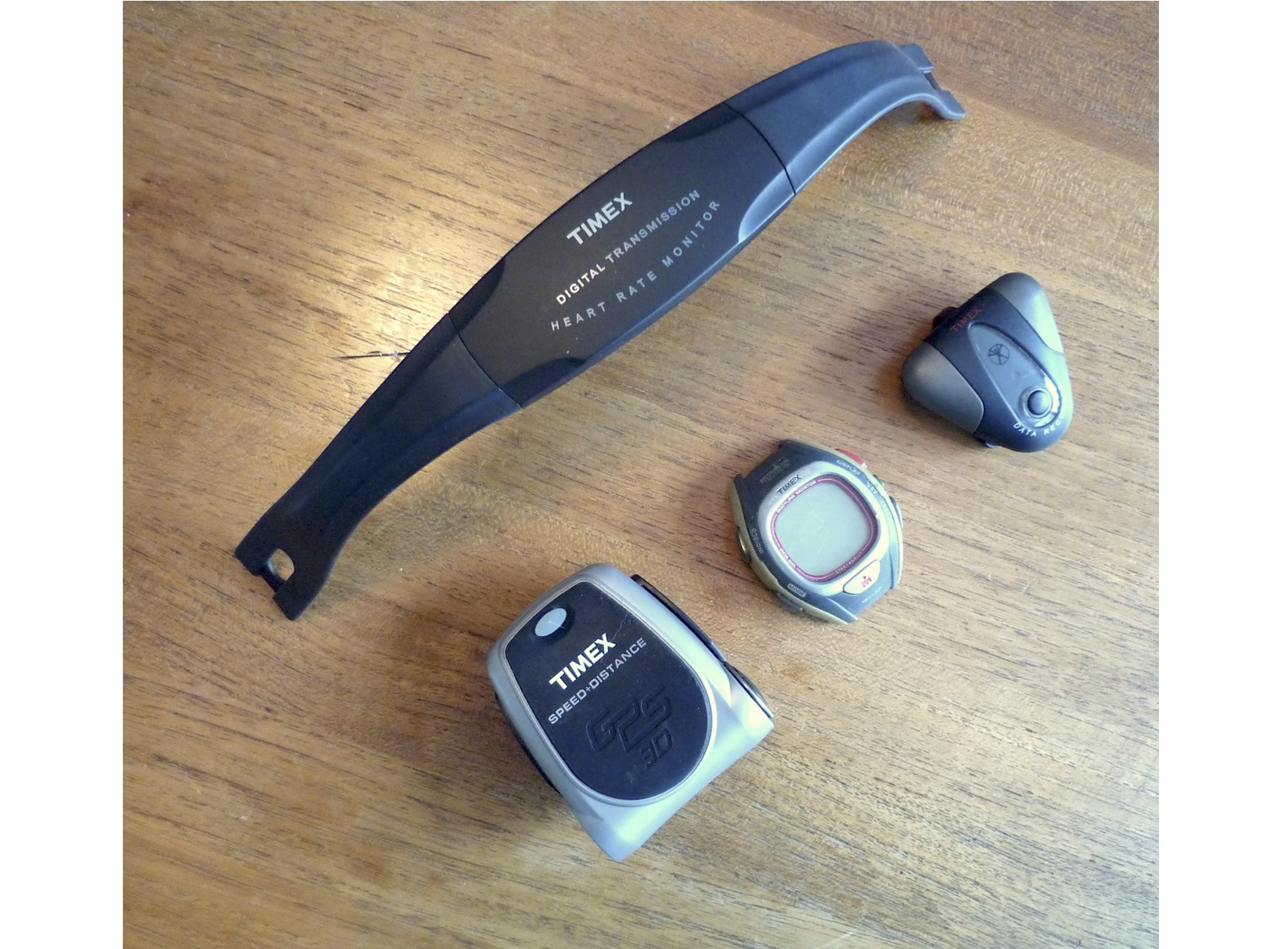
Figure 11: Timex BodyLink system: HR chest strap (top left); GPS receiver, watch data recorder.
Things got a little simpler when Garmin introduced the Forerunner 301 in 2004. The Forerunner 301 integrated the GPS receiver, display, and data processing and recording functions into one package, shaped a bit like a Vienna Finger cookie. It also received and displayed heart rate data from a wireless chest strap sensor. The receiver and display module was a bit awkward to wear on one’s wrist, but it worked just fine attached to a bracket (for easier reach) or thwart for paddling, as shown on my C-1 in Fig. 12. The rest, as they say, is history.
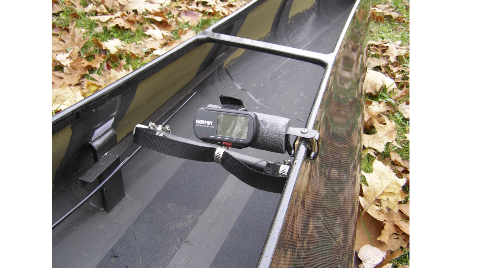
Figure 12: Garmin Forerunner 301 and C-1.
SUMMARY
In this installment of the Science of Padding series we presented an overview of the Global Position System. The simplified review of the mechanics of trilateration were presented. We also saw how developments in low-cost, energy-efficient electronics enabled the development and productization of mobile GPS systems for sport in the late 1990s and early 2000s. This was not an exhaustive overview of every innovation in the field, just a review.
So next time you’re out paddling, running, or hiking with your hand-held or thwart-mounted GPS receiver, pause for a moment and consider all of the things that make this aspect of your recreation possible. There’s a stunning amount of algorithms and engineering packed into feature-rich products that can now be had for less than $200 US. All enabled by science. Oh, and a little math, too.
V1.0
(c) copyright 2020, Shawn Burke. All rights reserved. See Terms of Use for more info.
- We’ll skip a lot of steps in this description that aren’t that important to the end user concerning carrier frequencies, modulation and demodulation, adjusting for variations in clock speed due to general relativity, code-locked and phase-locked loops, preambles and payloads, correlation a lot of math, etc. ↑
- Accurate to within about 1 second in 30 million years. ↑
- Since the receiver clock will continue to drift the synchronization process must be repeated, hence it’s best to think of it as a re-synchronization. ↑
- Note that there are several ways to make this calculation. Modern GPS receivers implement sophisticated signal processing (in the form of Kalman filters) that use some combination of Dopper, phase, and position fix data to estimate velocity. But the implementations vary vendor-to-vendor, and across models and product lines for even a single vendor. ↑
- Introduction to GPS: The Global Positioning System, Artech House Publishers, 2002 ↑
- Redin, Maria S., Marathon Man, B.S. and M.S. thesis, Massachusetts Institute of Technology, June 15, 1998. ↑
- “Cutting Edge Monitoring The Human Body,” World News Tonight With Peter Jennings, broadcast September 19, 1997. ↑