Part 32: Home on the Ranges

by Shawn Burke, PhD

Introduction

One of the perks of writing the Science of Paddling blog is email from readers. Emailers ask questions that motivate new articles. I was recently asked whether the power-to-weight ratio derived in Part 1: Tandem vs. Solo applied to sprint paddlers. Part 1 used dimensional analysis to derive the cubic relationship between speed and power. Underlying the analysis was an important assumption: the hulls were moving at steady speeds. Does the power-to-weight ratio apply when a hull is accelerating off the line for a 200m sprint? And what else can we learn by comparing accelerating versus cruising operating ranges?

Quite a lot, it turns out. And some of it may surprise you. We’ll begin by reviewing the paddled hull’s dynamic model derived in Part 24: Tales of Power.

Some of you may ask, why not simulate it all and be done with it? I’ve got nothing against simulation. When used appropriately simulation has tremendous value. But if you can write down a simple model of a system you can investigate so-called “limiting cases.” What happens when one quantity is large compared to the others? Or when it’s small? Do these represent operating ranges of the system encountered in real life? This type of investigation provides insight into what’s important in one or more system operating ranges. These insights inform what simulations to perform.

(Note that this post is organized like chapters in the upcoming Science of Paddling book. Detailed derivations appear at the end in an “Extra Credit” section for interested readers. And conclusions are bulletized in the “Take Aways” section.)

The Model

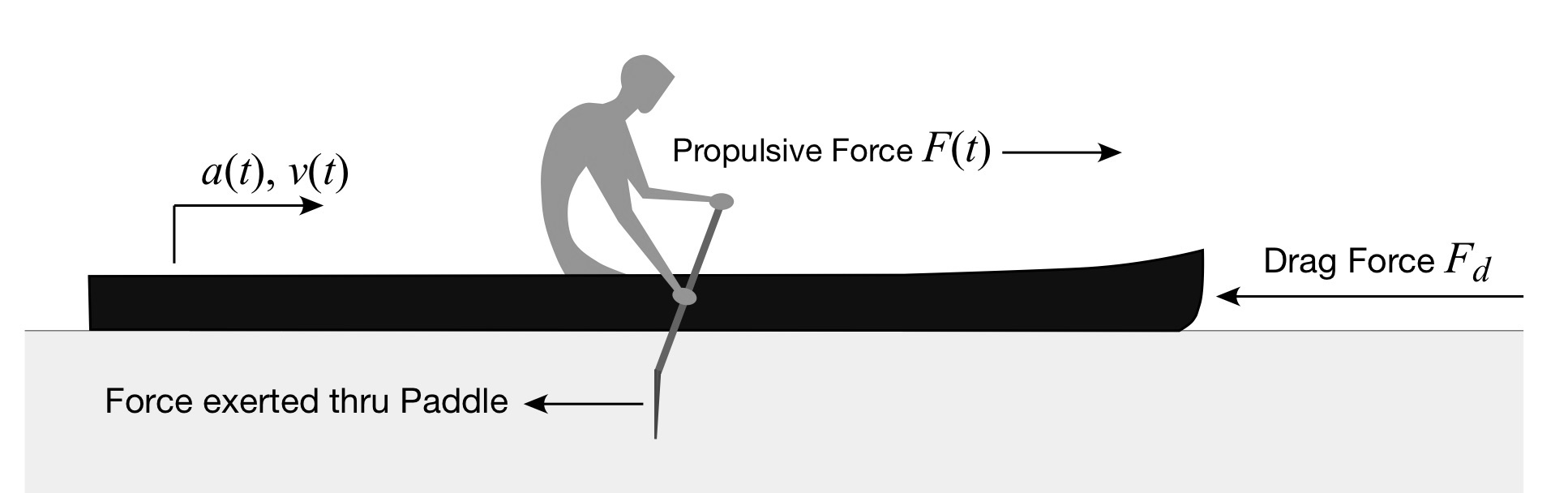
Figure 1: Forces acting on the hull/paddle system.

Consider the hull/paddler system depicted in Fig. 1. The paddler exerts a force through the paddle that results in a propulsive force F(t).^[1] The hull experiences a drag force F_d which opposes the propulsive force; since forces are vectors their directions are indicated by arrows in the figure. The hull moves with speed v(t) and acceleration a(t). Newton’s Third Law of Motion requires that these forces balance. Newton’s Second Law requires that the total force acting on the hull and paddler equal the change in their momentum. Since the hull and paddler’s mass m doesn’t change appreciably over time, the change in momentum equals the product of mass and acceleration. These requirements then yield the governing equation

$m\frac{dv\left( t \right)}{dt}=-{{C}_{D}}{{v}^{2}}\left( t \right)+F\left( t \right)$

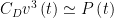
The acceleration a(t) is represented here as the time rate of change of the velocity v(t). This is written as the derivative of the velocity v with respect to time t, e.g., d/dt; derivatives are merely a quantity’s (here, velocity) rate of change with respect to a variable (here, time). This notation will be helpful in our analysis. The drag force as modeled as proportional to the velocity squared, which we derived in Part 26, and employed in Part 1 and Part 14. C_D is the drag coefficient derived in Part 26. Note that the drag force and propulsive force have opposite signs, which reflects how drag opposes the propulsive force.

Our governing equation embodies Newton’s Laws of Motion in a compact form using familiar real-world quantities: mass, velocity, drag, and paddling force. The math is just a compact language representing these concepts and observed phenomena.

Operating Ranges

Our governing equation lets us derive the power formula from Part 1 directly, rather than via dimensional analysis. We begin by multiplying both sides of the equation by the velocity v(t), and moving the drag term to the left-hand side,

$m\frac{dv\left( t \right)}{dt}v\left( t \right)+{{C}_{D}}{{v}^{3}}\left( t \right)=F\left( t \right)v\left( t \right)$

As we learned in Part 1, as well as Part 24: Tales of Power and Part 9: Power to the Paddlers, propulsive power P(t) equals the product of propulsive force F and hull velocity v. Consequently, the right-hand-side of the equation above is the propulsive power.

The first term in the equation above includes the acceleration, represented by the time derivative of velocity. When we’re cruising the hull doesn’t accelerate as much as when we are starting or changing speeds. So, for the steady speed case we’ll drop the first term in the equation.^[2] What we’re left with is the approximate relation between propulsive power and cruising velocity,

${{C}_{D}}{{v}^{3}}\left( t \right)\simeq P\left( t \right)$

This is the cubic relationship we derived in Part 1. Check! It’s nice to obtain the same result using two different methods. However, in Part 1 one we could only conclude that the power was proportional to the velocity cubed. Our new derivation lets us see that the proportionality constant is the drag coefficient. So, a sleeker hull requires less paddling power for a given cruising speed, and this proportionality between power and drag coefficient is linear.^[3]

Now what happens when the hull is starting from a stop, or accelerating to change gears? As you might expect we need to focus on the acceleration term in our power equation. We’ll assume that the hull velocity is either small compared to the acceleration, or that we’re traveling at a steady speed and the change in velocity from that speed is small compared to the acceleration.^[4] In this case the velocity cubed term will be small enough that we can neglect it in compared to the other terms,^[5] leading to the approximation

$m\frac{dv\left( t \right)}{dt}v\left( t \right)\simeq P\left( t \right)$

The left-hand side of this equation – the product of mass, acceleration, and velocity – can be written as the time rate of change of a quantity we encountered in Part 4: Shallow Water,

$m\frac{dv\left( t \right)}{dt}v\left( t \right)=\frac{d}{dt}\left[ \frac{1}{2}m{{v}^{2}}\left( t \right) \right]$

The bracketed term in this equation is the hull/paddler system’s kinetic energy, e.g., energy associated with motion. As a result, when acceleration is the dominant state variable for our hull/paddler system, before drag’s nonlinear dependence begins to dominate, we see that there is a new power to weight ratio,

$\frac{P}{m}\simeq \frac{d}{dt}\left( \text{Kinetic Energy} \right)$

This suggests that a for a given paddling power P a lighter team (less mass m) contributes to the system’s motion energy faster than a heavier team. Or for teams with the same mass, the team with greater paddling power will “jump” speeds faster. Compared to the steady-state power to mass ratio derived in Part 1, there are no fractional exponents. The relationship between power and mass is linear. This tells us that when accelerating the inertial term is initially dominant.

You may ask, what about when both acceleration and velocity are important? Aside from directly solving the nonlinear governing equation, or simulation, we can investigate a third limiting case. What if both velocity and acceleration are “small”?

When is a Nonlinearity Linear?

The drag force in our governing equation is linearly proportional to the drag coefficient CD, and nonlinearly proportional to velocity. This is because the drag force is proportional to the velocity is squared. If the drag force were linearly proportional to the velocity, then solving the governing equation in closed form^[6] would be a straightforward exercise. So, is a nonlinearity ever linear?

The question of linear versus nonlinear boils down to whether we want a solution that’s valid for all paddling speeds (a “global” solution) or one that’s valid for certain operating conditions (a “local” solution). As we saw above the governing equation can be simplified when the hull’s velocity is small compared to its acceleration, or when the inertial (acceleration) term is small compared to the nonlinear drag term. In the first limiting case we can solve the approximate governing equation using a calculus technique called integration, which is the inverse of differentiation. For the second limiting case we only need to use algebra, like we did in Part 1.

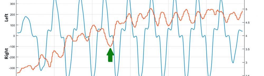
The operating condition we’re interested in next is embodied by the velocity trace in Fig. 2. Fig. 2 is a plot of kayaking paddle blade force (the blue curve) and hull speed (the red trace) as the kayak accelerates to a cruising speed. Note that the right ordinate ranges from 2 to 6 m/s rather than starting at 0. The velocity oscillations after about 227 sec indicate the hull accelerates and decelerates somewhat about an average velocity of about 4.8 m/s. The magnitude of these variations is around 10% of the steady state (average) speed.

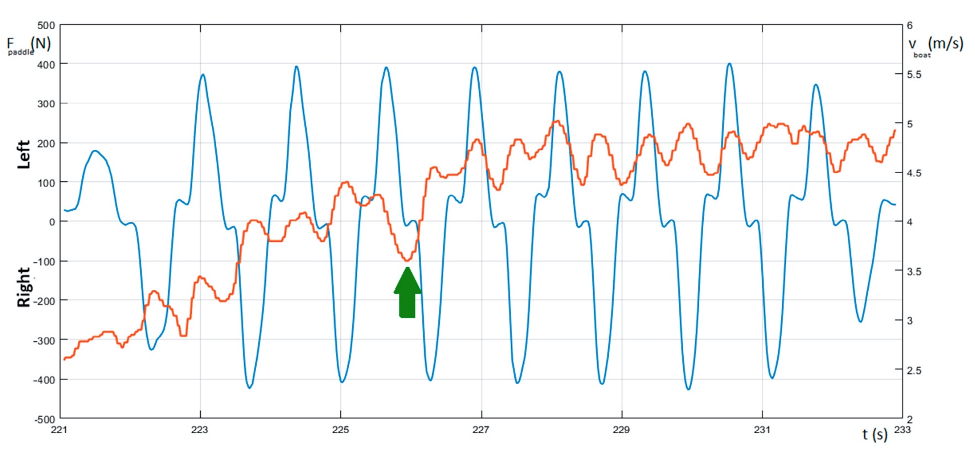
Figure 2: Kayak paddle force (blue) and the hull speed (red).^[7]

We can represent the velocity v(t) as the sum of an average velocity U₀ and smaller velocity oscillations u(t) via

$v\left( t \right)\equiv {{U}_{0}}+u\left( t \right)$

If we substitute this into our governing equation, use the fact that |u| << U₀ , and only retain the larger terms, our governing equation for a cruising hull simplifies to

$m\frac{du\left( t \right)}{dt}+bu\left( t \right)=f\left( t \right)$

where the constant b is defined in terms of the drag coefficient via

$b\equiv 2{{C}_{D}}{{U}_{0}}$

You’ll find a detailed derivation in the Extra Credit section.

The approximate governing equation for a cruising hull has a remarkable property: it’s linear. How could this be so?

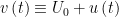
The simplest way to understand this is to look at the drag force’s quadratic nonlinearity, shown in Fig. 3 over velocity range from 0 mph to 7 mph. At four velocity values – 1, 2, 4, and 6 mph – you’ll find a straight-line approximation to the quadratic curve. I chose the local tangent; you could equally as well use the local secant. Notice how good the local straight-line approximations are around each of these four set points. If we extend any of these tangent lines, we’d see that none would make good global approximations. But they are surprisingly good local approximations.^[8]

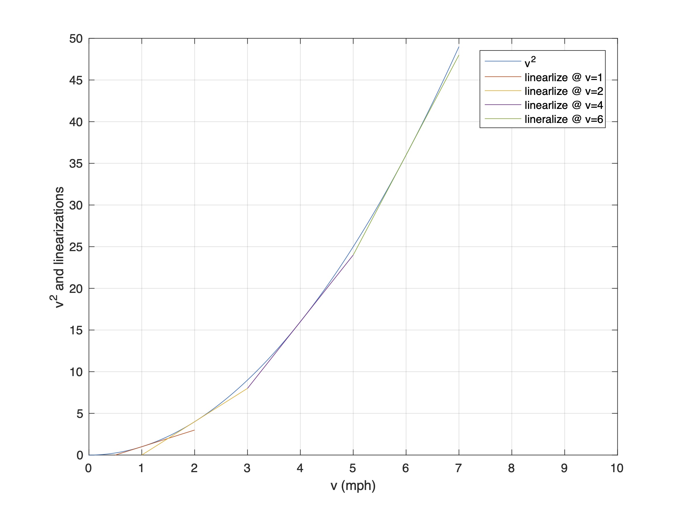
Figure 3: Quadratic and four local linear approximations.

One approximation’s local fidelity is shown graphically in Fig. 4 for the v = 2 mph set point. Over a 0.5 mph span the tangent is an excellent linear representation of the quadratic.

Figure 4: Quadratic and linear approximation about x=2.

So over local operating ranges – cruising, with sufficiently small velocity variations about the average velocity^[9] – the quadratic drag force simplifies to a linear drag force. The resulting governing equation is locally linear. What does this imply?

One important property of linear systems is superposition. Superposition means that if you have the solution to a governing equation for one input, and the solution to the governing equation for another input, if the inputs are combined then the resulting solution is merely the sum of the two previous solutions.

Do paddled hulls have more than one input when cruising? If there are two or more paddlers in the hull, the answer is yes. Each i-th paddler provides a propulsive force F_i(t). If these paddlers in a cruising hull paddle in sync the average hull speed will equal a certain value; note that averaging is a linear operation. If these paddlers paddle out of sync… the average hull speed will be the same, consistent with the assumptions above.

Obviously padding out of sync may entail hydrodynamic penalties if the hull surges, rolls, or bounces. And in tandem and quad kayaks or dragon boats paddling out of sync might lead to cracked paddles and hostile teammates. But barring these complications, when at a cruising speed with small speed variations, paddling in sync might not be the hard and fast requirement we’re all ingrained to do. One more reason I need to revisit Part 2!

Extra Credit

As presented in Equation (7), we represent the velocity v(t) as the sum of an average velocity U₀ and smaller velocity variation u(t) via

$v\left( t \right)\equiv {{U}_{0}}+u\left( t \right)$

The velocity squared is then

${{v}^{2}}\left( t \right)={{\left[ {{U}_{0}}+u\left( t \right) \right]}^{2}}=U_{0}^{2}+2{{U}_{0}}u\left( t \right)+{{u}^{2}}\left( t \right)$

Since we assume that the velocity variation is small compared to the average velocity,

${{v}^{2}}\left( t \right)\simeq U_{0}^{2}+2{{U}_{0}}u\left( t \right),\text{ }u\left( t \right)\ll {{U}_{0}}$

The inertial term, which is based on the rate of change of the velocity, is simply

$m\frac{dv\left( t \right)}{dt}=m\frac{d}{dt}\left[ {{U}_{0}}+u\left( t \right) \right]=m\frac{du\left( t \right)}{dt}$

because the rate of change of the constant average speed is zero. The governing equation is then

$m\frac{du\left( t \right)}{dt}=-{{C}_{D}}U_{0}^{2}-2{{C}_{D}}{{U}_{0}}u\left( t \right)+F\left( t \right)$

We can also define our force F(t) in terms of a constant average force, and variations of this force f(t),

$F\left( t \right)={{C}_{D}}U_{0}^{2}+f\left( t \right)$

The constant term is merely the average propulsive force required to maintain an average velocity U₀. In essence we are re-writing our governing equation about a set point.

We define a new constant b in terms of the drag coefficient and average velocity,

$b\equiv 2{{C}_{D}}{{U}_{0}}$

Substituting into our “cruising set point” governing equation yields Equation (8)

$m\frac{du\left( t \right)}{dt}+bu\left( t \right)=f\left( t \right)$

QED

Take-Aways

The cubic relation between paddling power and hull speed was derived using the equation governing a paddled hull’s motion. This approximation was shown to be valid when the hull was cruising.
When a paddled hull is accelerating the ratio of paddling power to the hull and paddler’s mass is proportional to the rate of change of the system’s kinetic (motion) energy.
When the hull is cruising, with “small” changes in hull velocity, the nonlinear governing equation yields a linear approximation.
Linear systems embody the property of superposition: If their input can be represented as a sum of inputs, then the response to the sum of these inputs equals the sum of the responses to each input individually.
Superposition implies that for cruising hulls the constraint of paddling in sync might be less important than we’d thought. That said, paddling out of sync may entail a hydrodynamic penalty if the hull surges, rolls, or pitches. The hydrodynamic impact of various paddling schemes is not captured in the governing equation. Be careful out there! The paddle you strike might be your teammate’s.

References

Vincenzo Bonaiuto, Giorgio Gatta, Cristian Romagnoli, Paolo Boatto, Nunzio Lanotte, and Giuseppe Annino, “A Pilot Study on the e-Kayak System: A Wireless DAQ Suited for Performance Analysis in Flatwater Sprint Kayaks,” Figure 9 pp. 13, Sensors 2020, 20, 542; doi:10.3390/s20020542.

The analysis applies equally well to kayaks, SUPS, tandem hulls, dragon boats, outriggers, and other paddled craft. ↑
Yes, there’s always acceleration or deceleration, even when cruising, due to the time variation of the paddle force. We’re just focusing on a particular operating range where acceleration has a small effect. ↑
Perhaps that’s why racers pay big bucks for faster hulls? ↑
The latter case is left as an exercise to the reader; you can borrow from the analysis in the Extra Credit section. ↑
Yes, it’s an approximation. ↑
This means we could write down the solution on a sheet of paper, rather than having to solve it using numerical simulation. ↑
from Vincenzo Bonaiuto, Giorgio Gatta, Cristian Romagnoli, Paolo Boatto, Nunzio Lanotte, and Giuseppe Annino, “A Pilot Study on the e-Kayak System: A Wireless DAQ Suited for Performance Analysis in Flatwater Sprint Kayaks,” Figure 9 pp. 13, Sensors 2020, 20, 542; doi:10.3390/s20020542. Many thanks to Nunzio for granting me permission to reproduce the figure. ↑
This type of local linearization was used to design linear feedback controllers for various nonlinear systems. ↑
Whatever that average speed may be! ↑

The Science of Paddling

The intersection of physics, physiology, and paddle sport