by Shawn Burke, Ph.D.

INTRODUCTION

I heard a rumor that you could use a bicycle cadence sensor as a stroke rate sensor for paddling. Naturally, I was intrigued. And puzzled. Intrigued, because some paddlers contend that stroke rate is an important parameter that can be used in training and racing^[1]. And puzzled because the bike cadence sensors I was familiar with comprised a magnetic sensor attached to the bike frame, and a small magnet attached to the crankarm. When the chainring rotated the magnet passed by the sensor, closing a switch. Associated electronics sensed this closure; one could infer that downstream electronics and software counted closures, divided this by time, and computed cadence, e.g. the number of times you turned over the chainring per minute. So where do you mount all that stuff on your paddle?

Cadence sensors – and sports sensor technology in general – have progressed a bit since I last fiddled with setting up a bike cadence sensor. Bike cadence sensors no longer need fixed sensing elements on the bike frame nor fiddly magnets on the crankarms; ditto for bike speed sensors. Nowadays, these sensors are built using solid state (aka, MEMS, or Micro-Electro-Mechanical Systems) inertial sensors^[2] , packaged in monolithic housings that can be readily attached to bicycle crankarms. And to paddle shafts, too.

So in this installment of the Science of Paddling series we follow the lead of my late father. Dad was adept at using tools for lots of things they were never designed to do (“No grinder? But you’ve got a drill!”) and never losing any fingers in the process. We’ll investigate whether one of these newfangled MEMS-based bike cadence sensors can measure your stroke rate. And if so (or if not), why?

GIVE IT A WHIRL

Fortunately, I had a cadence sensor that I’d used to soup up a spin bike to make it “smart.” The sensor is mounted to the crankarm as shown in Fig. 1; the yellow sticky note is there only to provide visual contrast between the black sensor housing and the black crankarm. The sensor is attached using a high-tech rubber band, which makes it easy to mount and unmount.

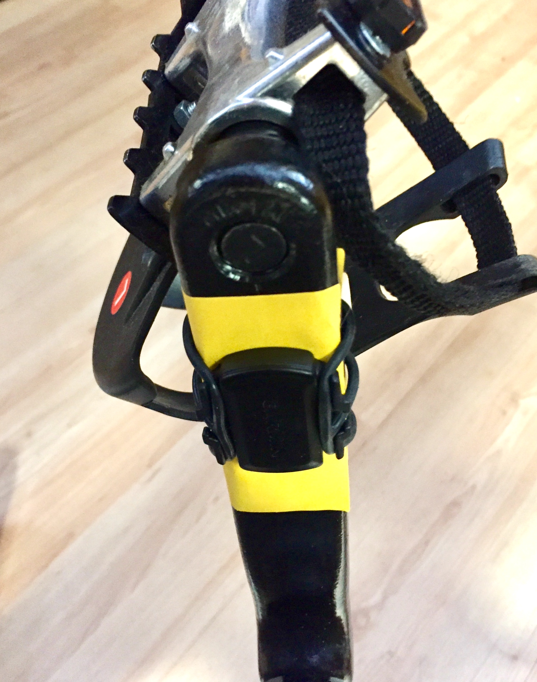
Fig. 1: Cadence sensor on spin bike crankarm.

The cadence sensor is wirelessly connected to a sports watch (or bike computer). Setup is simple, and after pairing the sensor to the watch you can ride the bike and track your cadence while sweat pours off your brow. You can also save the data for post-workout analysis.

Since we’re interested in using this sensor for paddling, I unmounted it from the spin bike and mounted it to the paddle shaft on my canoe ergometer, as shown in Fig. 2. I’m a canoeist, which in North America means I use a single-bladed paddle. The sensor was already paired with my sports watch, so I turned on the watch and started paddling, fully expecting to see cadence numbers on the display.

I was sorely disappointed.

I tried paddling fast, slow, and everything in between. No data was forthcoming from the sensor; just an empty space in my sports watch’s cadence data field. I was able to sporadically coax “real” cadence numbers from the sensor if I adopted ludicrously exaggerated stroke mechanics, swinging the paddle out to the side and recovering well above my shoulder. Even then the data seemed to have little to do with my stroke – when there was actually data forthcoming.

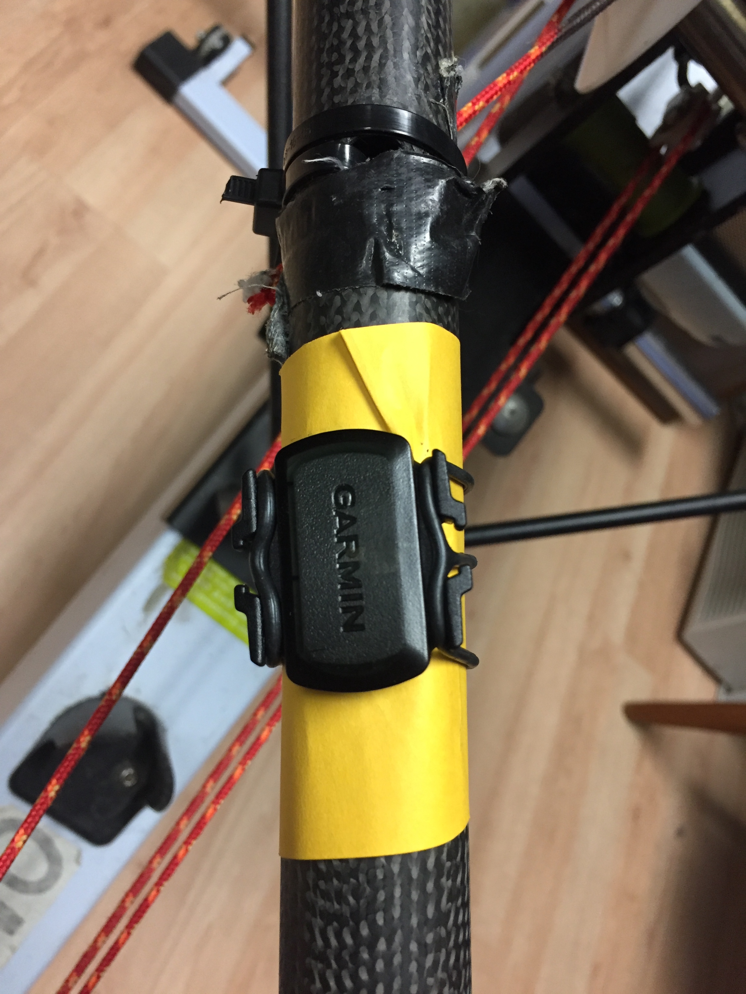
Fig. 2: Cadence sensor on canoe erg paddle shaft.

My gyrations reminded me of a kayak stroke. Or at least a kayak stroke performed by me, a person unskilled in the art of the double blade. It dawned on me that perhaps the bike cadence sensor would be more suitable for kayakers. I went to the garage and brought back my best facsimile of a kayak paddle: an old broom handle. I mounted the cadence sensor on my super high-tech carbon fiber^[3] paddle shaft, as shown in Fig. 3, and tried the experiment again.

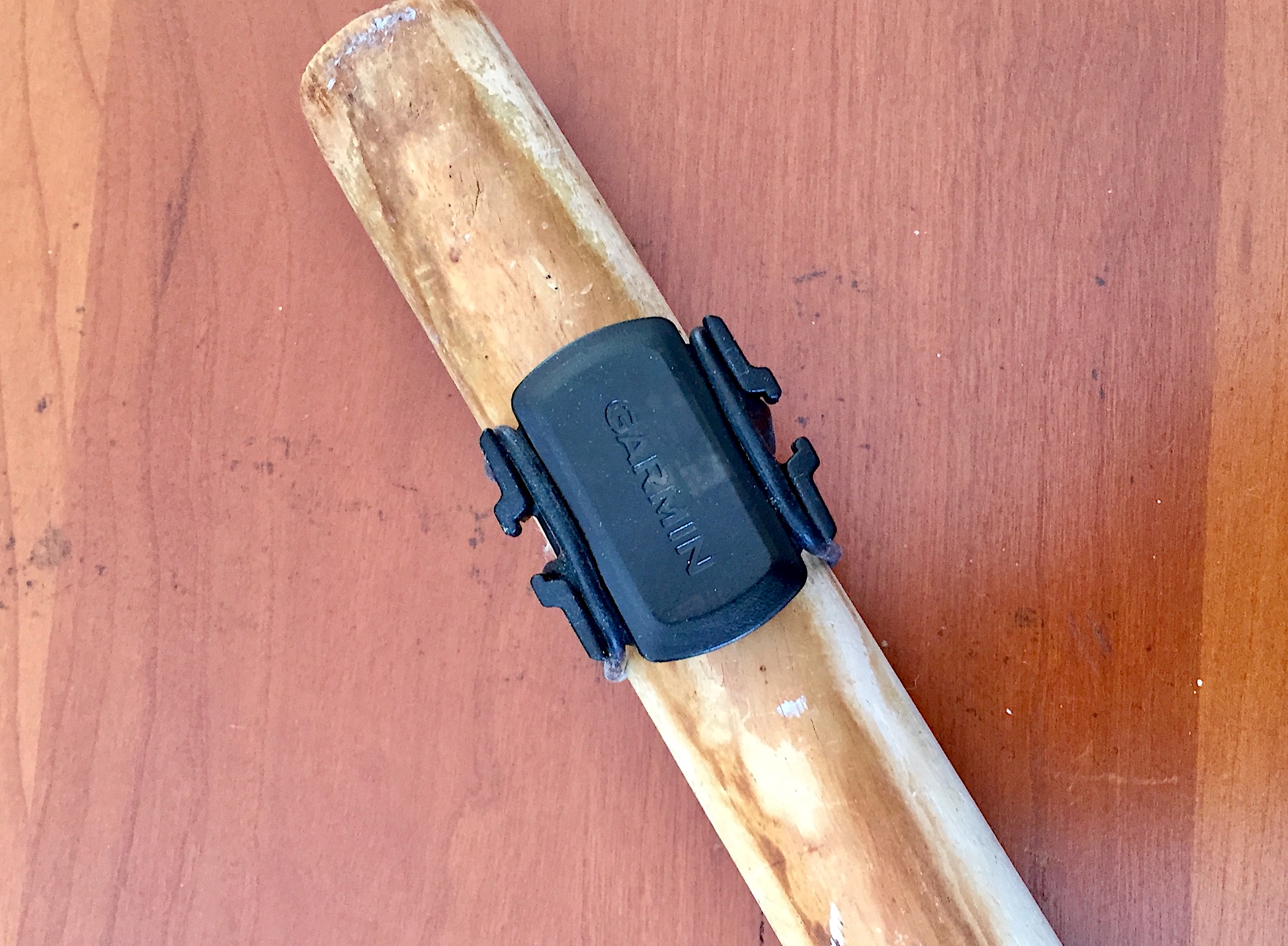
Fig. 3: Cadence sensor on “kayak paddle shaft.”

Much to my surprise and pleasure, I got data! An example is shown in Fig. 4 (not captured by me: I was busy “paddling” with my broom stick).

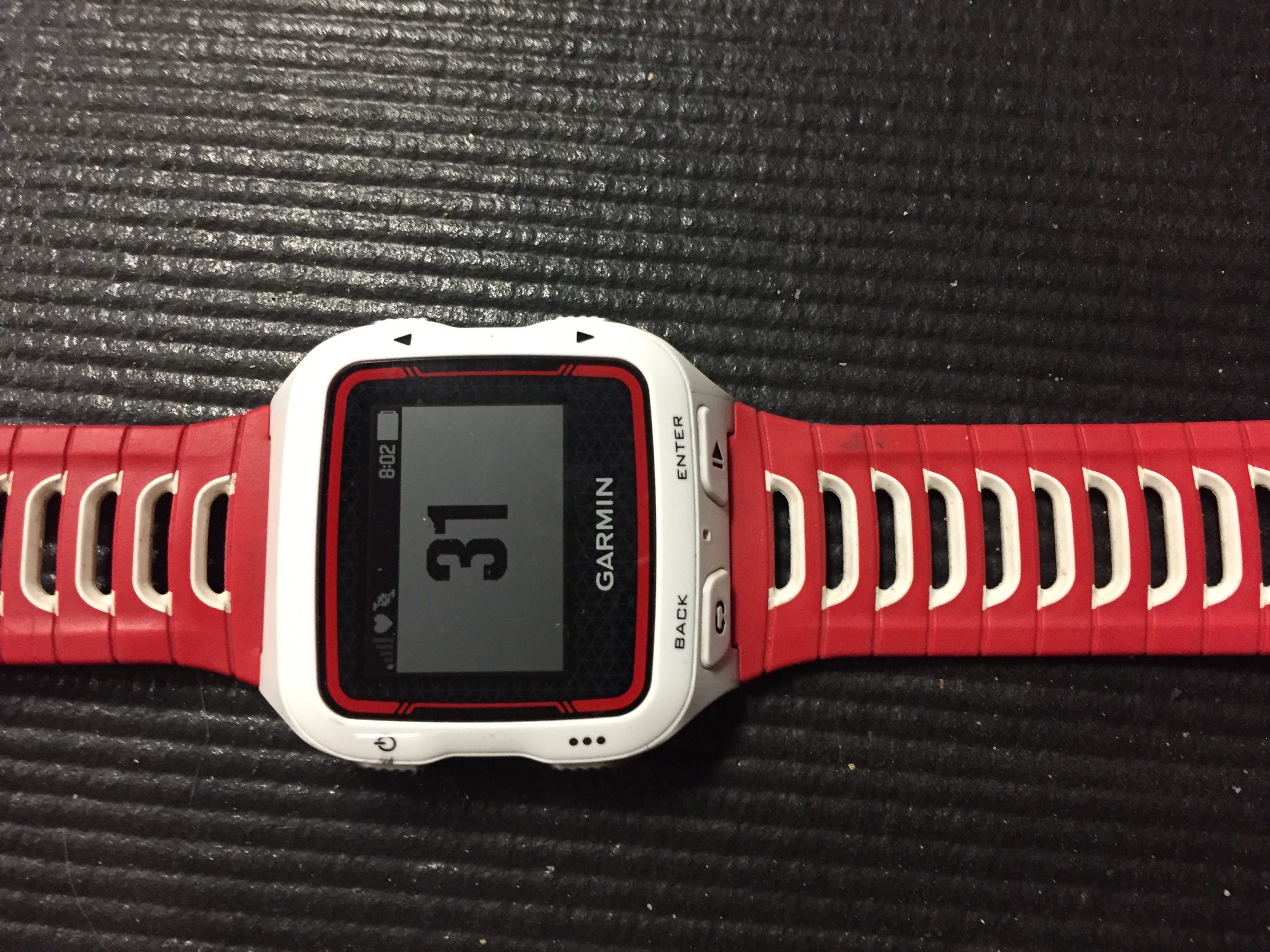
Fig. 4: Cadence data (SPM) example, “kayak” case.

The data values I saw were proportional to the cadence of one “blade” (e.g., the end of the broom handle) rather than the stroke rate of the entire left-right paddling motion. If you want that number just multiply by two. Data sometimes appeared intermittently, and it took a while after starting for the sensor to actually start spitting out data. But it worked. More or less. I’ll call it a qualified success, qualified no doubt by my lack of double-blade skill or finesse.

So if you’re interested in whether or not you can use a bike cadence sensor for measuring paddling stroke rate, there’s your answer. But if you’re interested in the why – and if you’re reading The Science of Paddling, I’d be surprised if you weren’t – then read on.

CYCLES AND CYCLOIDS

Sitting there, swinging my “kayak paddle” in what approximated an actual kayak stroke made me realize that the “blade” ends were describing roughly circular orbits. And what path is described by a bike cadence sensor mounted on a spin bike crankarm? A circle. It was starting to make sense. But would it work on the water, when the sensor is also moving forward as well as describing a circular pattern?

I’ve used the cadence sensor on my road bike, and it works great. As the chainring spins on a moving bike a fixed point – like the mounting location of a cadence sensor on a crankarm – when seen by a stationary viewer, describes a curve called a “cycloid.” You can prove this to yourself by taking a can, taping a piece of chalk to it, and rolling the can alongside a wall (or blackboard). The pattern it marks as you roll the can looks like the blue curve in Fig. 5. A cycloid.

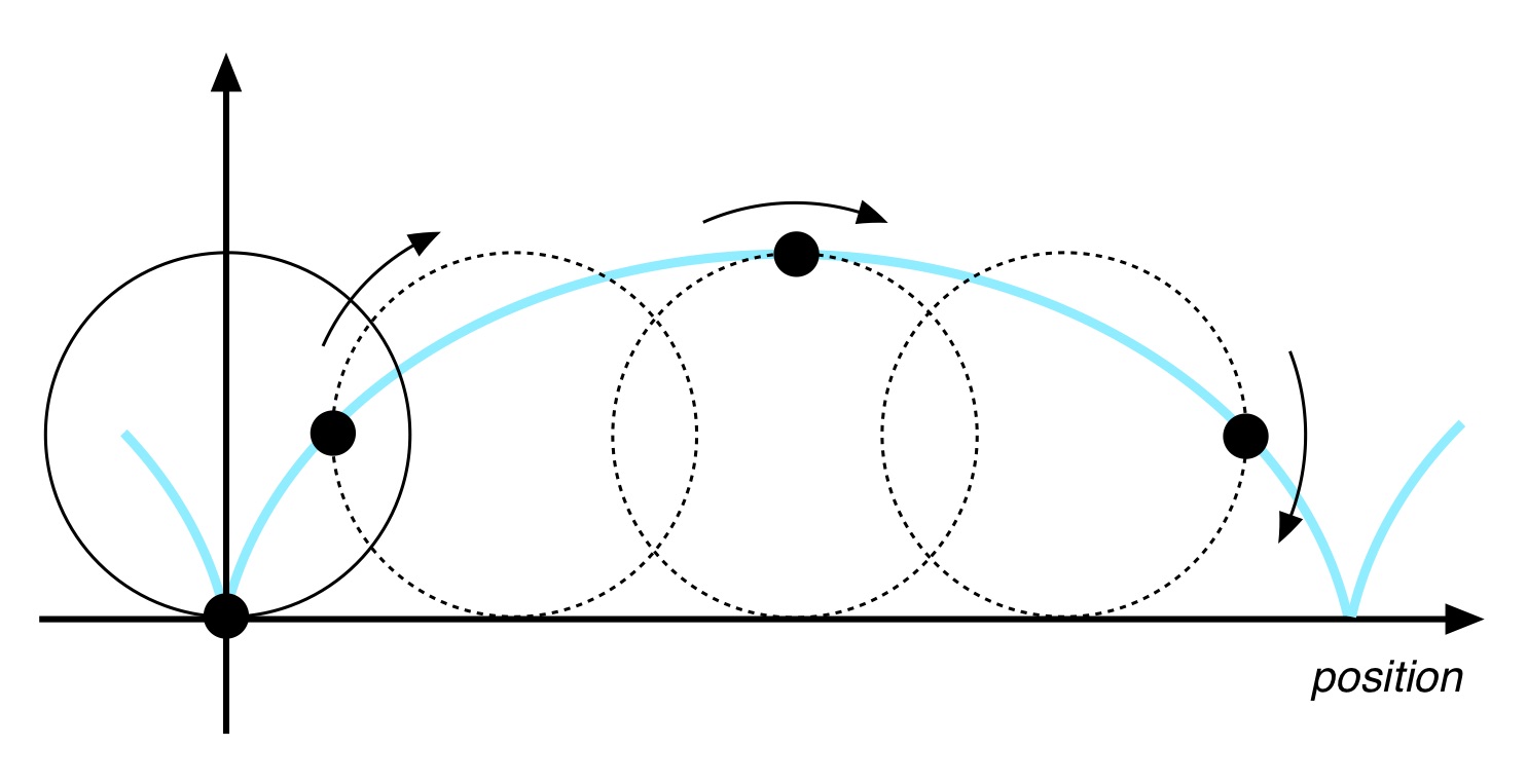
Fig. 5: Cycloid.

Does a kayak paddle describe this path as you paddle? If so, from the paddler’s reference frame the paddle will be moving in a circular pattern; from the perspective of a stationary viewer it will look like a cycloid. Rather than reinvent the wheel (so to speak) I remembered some fantastic time-lapse photos of a kayaker with a paddle covered in LEDs. These photos, taken by Stephen Orlando, can be found at motionexposure.com – check out all of his incredible shots (and purchase a few while you’re at it!). Fig. 6 is a time exposed ¾ view of a kayak paddle’s LEDs. Following the edge of the pattern you can see the dip at the catch, and the rise of the recovery after the power phase followed by the arc of the blade. The pattern is a pretty fair representation of a cycloid. Check.

By contrast, Fig. 7 includes analogous traces of a canoe paddle, similarly equipped with an array of LEDs. The shape reminds me a bit of a synthesizer filter’s ADSR (Attack-Decay-Sustain-Release) curve. You can discern the power phase placement, recovery, and reach for the next catch. But this stroke clearly does not describe a cycloid. Thus the canoe stroke, from the perspective of the paddler, does not subtend a circle. Which appears to be why I didn’t get any data when using the bike cadence sensor with my canoe ergometer.

Fig. 6: Kayak paddle path over distance. [photo: Stephen Orlando]

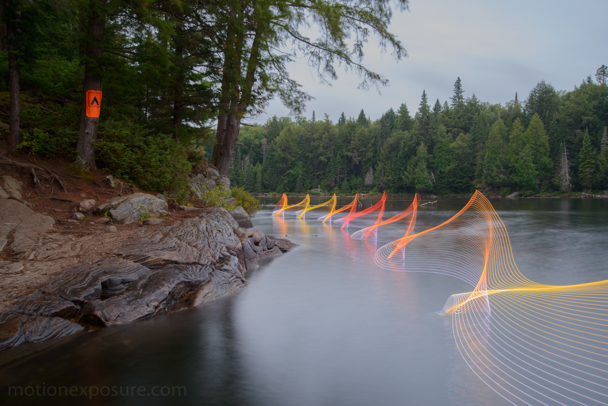
Fig. 7: Canoe paddle path over distance. [photo: Stephen Orlando]

Having established that the kayak stroke subtended a circular / cycloid path as a function of the observer’s location, I naturally started doing all sorts of tests with the device. The canoe stroke in three dimensions kinda looks like a folded oval; an oblong Salvador Dali pancake if you will. Did the bike cadence sensor have a perferred orientation of the circular path traced by the device?

To answer these questions I investigated the sensor’s performance in a controlled environment. I taped the sensor to my turntable, as shown in Fig. 8. This is a direct-drive turntable that can be hand-rotated. I studied the sensors’ response when the turntable’s platter was oriented vertically (as in Fig. 8), or in the more familiar horizontal orientation.

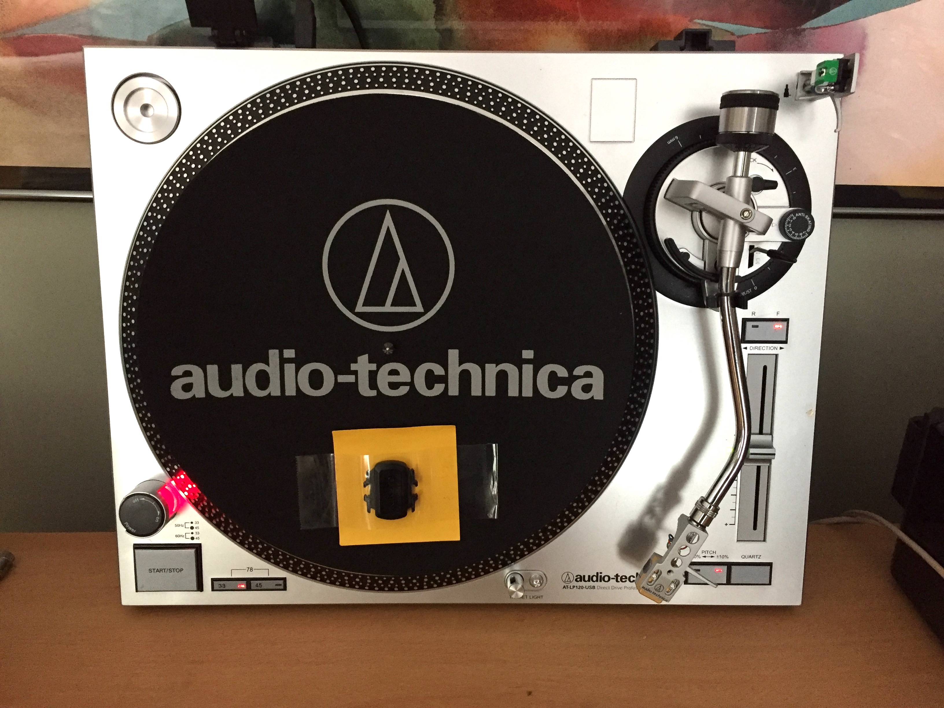
Fig. 8: Cadence sensor taped to turntable.

When oriented vertically the bike cadence sensor produced data immediately and consistently. An example is shown in Fig. 9. Note that the value does not correspond to any of the “traditional” turntable speeds of 33rpm or 45rpm since the direct drive motor did not have enough torque to spin the platter when oriented vertically; I had to spin it by hand. This orientation matches the orientation when the sensor is mounted on a bike crankarm. Check.

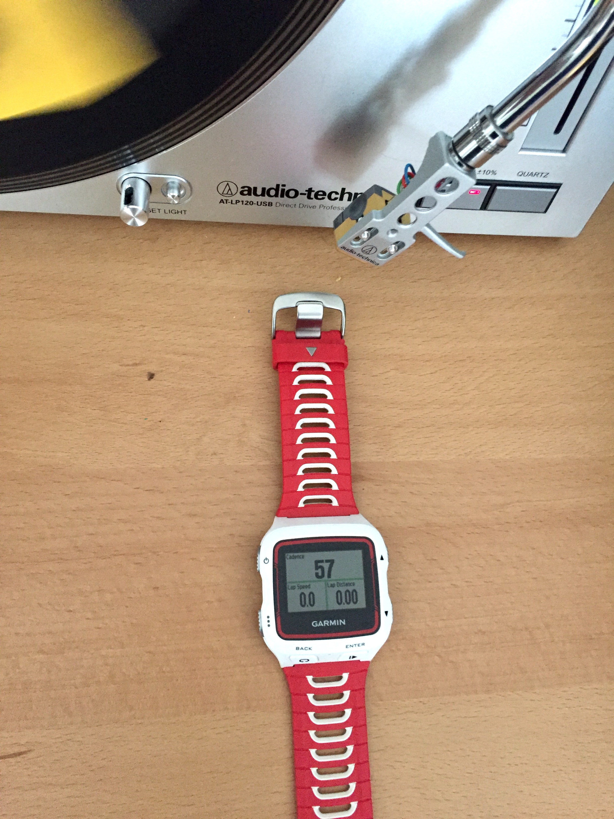
Fig. 9: Cadence data, turntable vertical.

I next tested the sensor when the turntable was placed flat on a table, i.e. with the platter horizontal, as shown in Fig. 10. Since the turntable was designed to spin in the horizontal plane I was able to run it at 33rpm. The bike cadence sensor did not produce any data in this orientation, as shown in the sports watch’s blank cadence field. What is it about the bike cadence sensor that caused it to produce data when spun in a vertical plane but not in a horizontal plane? Did this have something to do with the sensing element housed within the device? Well yes; it does. And to understand why we’ll first look at why one might use an accelerometer, i.e. a sensor that directly measures acceleration.

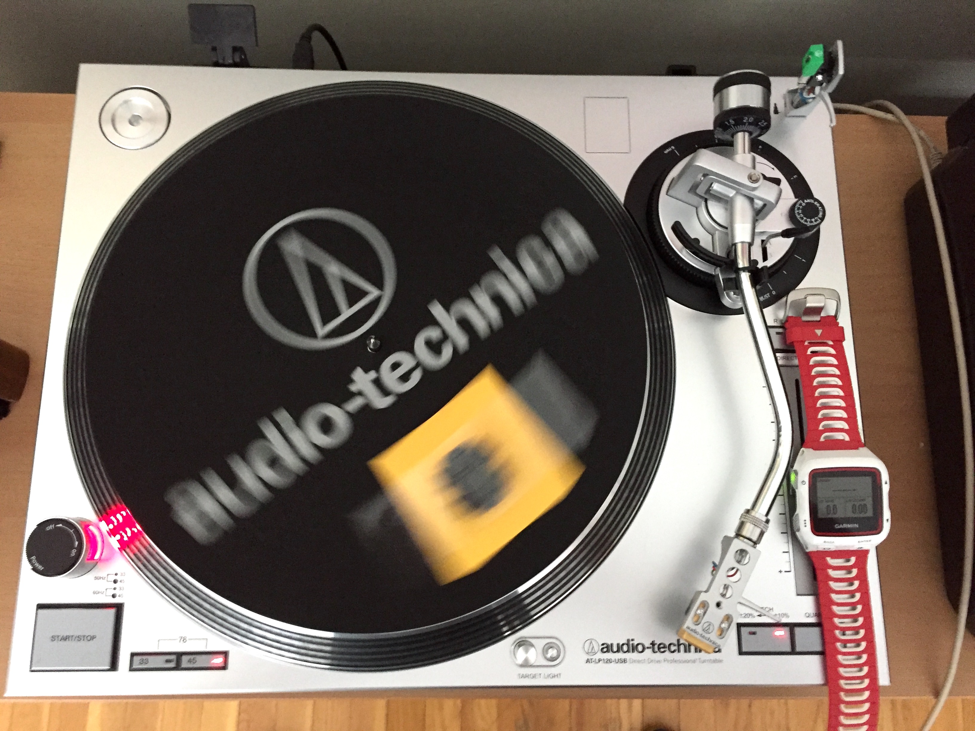
Fig. 10: Cadence data, turntable horizontal.

OK, GREAT. BUT WHY?

So why use an accelerometer in the first place? Isn’t there some other way to measure stroke rate? Of course there is. You could count your strokes while using a watch or a timer, and when the timer reaches one minute note the number of strokes you’ve counted then start counting again. That works but gets a bit tedious. The real time cadence “display” would be your thoughts. And “downloading” the data would entail remembering your stroke counts and writing them down when you’re done.

Alternatively, you could use a video camera, film your workout, and count strokes. Most digital cameras have an accurate time base that would facilitate computing cadence. But unless you write image processing software to (reliably and accurately) count strokes from the video images you’d be limited to post-workout analysis. Other approaches I can think of are best termed “R&D projects.” But… We already have accelerometer-based cadence sensors.

Since this is a Science of Paddling article, we’re also interested in another why: how do accelerometers work, and why didn’t they work in both turntable cases described above? To answer that we will consider how MEMS accelerometers are built and operate. The acronym MEMS indicates that these devices are Mechanical in nature – the second ‘M’ in MEMS does after all mean Mechanical – and have an Electrical component (from the ‘E’). MEMS are made up of elements between 1 and 100 micrometers in size (hence ‘M’ for Micro). They are produced using semiconductor device fabrication techniques that entail the deposition of material layers, patterning by photolithography, and etching to produce the mechanical elements. Signal conditioning electronics are produced alongside the mechanical structures; many modern devices include digital electronics for processing the sensed signal data. An exemplary device made by Analog Devices, Inc. is shown in Fig. 11 in a ¾ view.

The centipede-like structure in the background comprises a rectangular silicon mass centered among numerous parallel flexures. The mass can move in one direction parallel to the plane of the device, constrained by the flexures. The flexures are bendable beams, suspending the moving mass over the substrate base yet only allowing the mass to move in one direction: parallel to the substrate. As a result this sensor will respond to accelerations in the direction coincident to the long axis of the suspended rectangular mass, e.g. the direction in which the beam flexures are bendable. The beam flexures keep the mass from moving in response to accelerations perpendicular to the substrate; the beam flexures are stiff in that direction and hold the mass down. Ditto for accelerations in the direction parallel to the lengths of the beam flexures. Consequently this is a “single-axis” accelerometer, responsive to accelerations in only one direction.

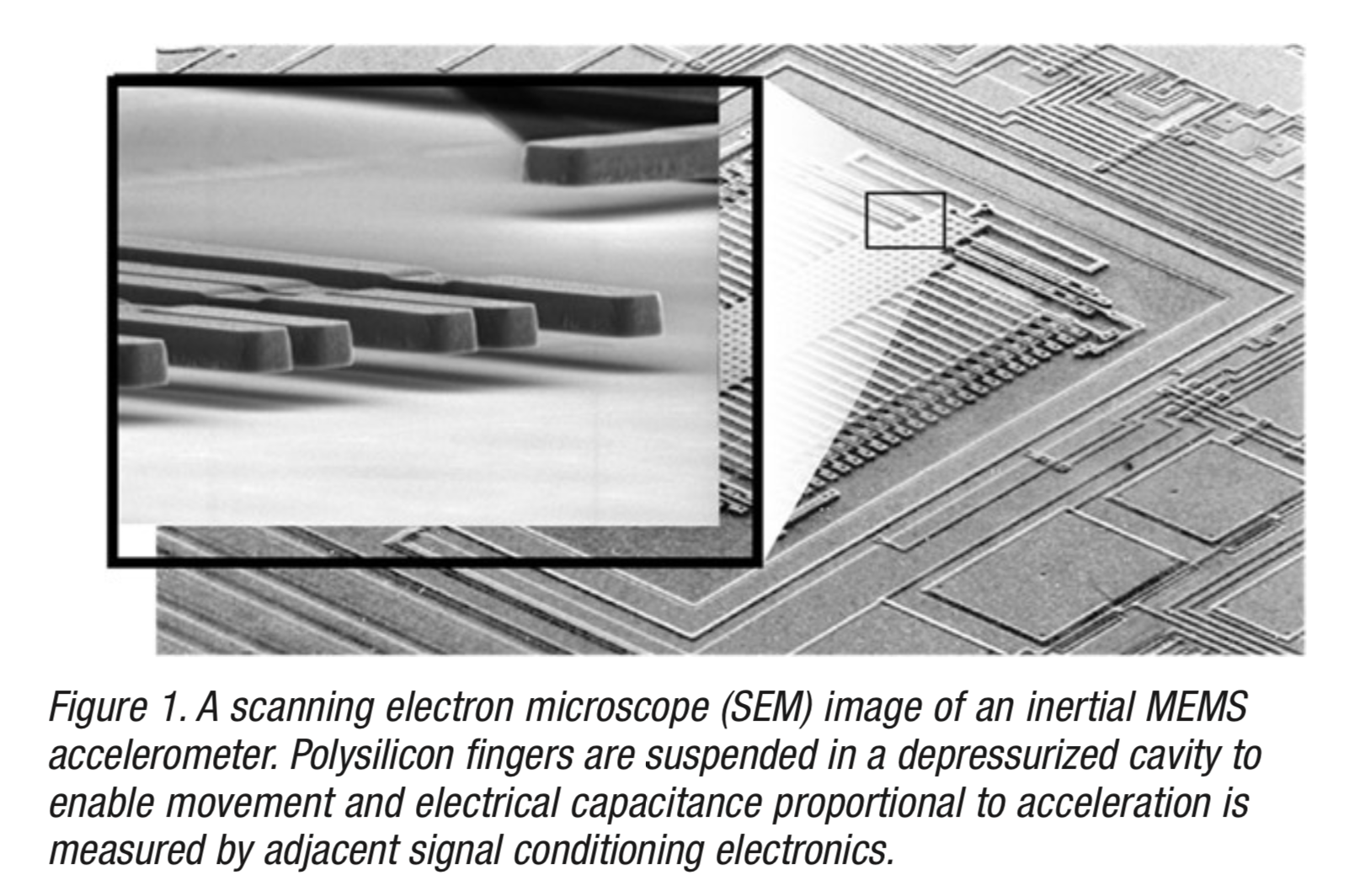
Fig. 11: SEM image of MEMS accelerometer. [from Ed Spence, “What You Need to Know About MEMS Accelerometers for Condition Monitoring”, Analog Devices, Inc. TA14725-0-7/16]

We can idealize a 1-D MEMS accelerometer as a mass placed atop a spring in the form of a beam, as shown in Fig. 12. In the figure the spring is attached to a rigid base, like the substrate in Fig. 11. The idealized device is analogous to your head and neck when you’re sitting in a car, where your head is the mass and your neck is the spring. When your car is moving at a steady speed – e.g., not accelerating – your head and neck are stationary in the car’s frame of reference, keeping a fixed distance from the seat’s head rest. When you press on the accelerator to move forward your head moves back toward the head rest. Who knew that you carry an accelerometer around with you all day long?

Elements labeled ‘1’ and ‘2’ in Fig. 12 are electrode “plates” parallel to the suspending beam. When the mass moves in response to an acceleration it moves toward one electrode, and away from another, as shown in the second figure. This is how your head moves toward a car’s head rest when you accelerate forward. MEMS accelerometers operate capacitively to determine acceleration. From high school physics you may recall that plates have an electrical capacitance inversely proportional to the distance between plates. We’ll utilize this in Appendix A to derive the governing electrical equation for this idealized MEMS device. But first, how does inferring this distance help us determine acceleration?

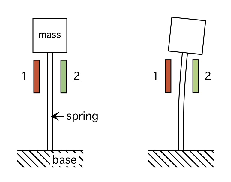
Fig. 12: Accelerometer concept.

We can show this readily using the governing equation for a spring-mass system. For a mass m, and beam with bending spring stiffness k, when the mass moves a distance x any sophomore mechanical engineer will tell you that

where x’’ denotes the second time derivative of displacement, i.e. the rate of change of the rate of change of displacement, or the rate of change of the mass’ velocity. Writing the acceleration as a and substituting, then solving for the acceleration gives

In other words, if we measure the displacement x of the mass then our measurement is linearly proportional to the acceleration a. (Analogously, if you measured your head-to-head rest distance in your car – and knew the mass of your head and the spring stiffness of your neck – you could infer your car’s acceleration.)

Notice that we’ve limited the mass to only move in one direction. The MEMS accelerometer shown in Fig. 11 is similarly constrained. The springs suspending the mass in this device are designed to move in one direction, a so-called parallel motion flexure. This means the device will sense acceleration in the direction parallel to the plane defined by the substrate, along the long axis of the central rectangular mass. It will not sense acceleration out-of-plane, nor in the direction parallel to the long axis of the flexures.

Sound familiar? Recall that when we mounted the cadence sensor to the turntable and tried to get data when the turntable was spinning horizontally, there was no data output? While I don’t know anything specific about the internals of the bike cadence sensor, one can infer that it comprises a 1-D MEMS accelerometer with a sensing axis lying in the plane of the turntable (or of the chainring) rather than perpendicular to it.

But what acceleration is being measured to infer cadence? Note that you can ride a bike at a steady speed – i.e., not accelerating, like on a spin bike – and turn the crankarm at a steady cadence – i.e., no angular acceleration, just spinning at a constant angular velocity – and still get cadence data output from the sensor. MEMS accelerometers measure acceleration. Where’s the acceleration in that case?

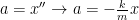
Let’s again consider the simplified MEMS sensor from Fig. 12, but now in four different orientations as shown in Fig. 13. An arrow is also shown depicting the acceleration due to gravity since we’ll be using our cadence on the Earth. (Should you question whether gravity is indeed an acceleration, and not a force, please see to Appendix B for an explanation.)

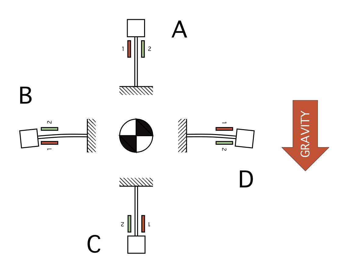
Fig. 13: Idealized accelerometer rotating in a gravitational field.

These four positions are labeled ‘A’, ‘B’, ‘C’, and ‘D’, respectively. At both the top and bottom positions A and C the mass/beam system is aligned with gravity. Consequently, the beam does not deflect toward either capacitive plate 1 or 2; the acceleration due to gravity is perpendicular to the systems’ direction of flexural motion. But at positions B and D the beam deflects owing to gravity acting on the sprung mass. At position B the beam is deflected toward plate 1, while at position D it bends toward plate 2. This change in sign can be used to disambiguate acceleration due to gravity vs. acceleration due to speeding up or slowing down your cadence. If the idealized acceleration sensor were mounted so that it could rotate as suggested in Fig. 13, then a non-zero angular acceleration (or deceleration) of the chain ring would always deflect the beam in one direction. The total acceleration acting on the sensor is the sum of all accelerations present, so the measured voltage would show the change in sign (or amplitude) due to gravity cyclically. This cyclical change can then be used to determine cadence since it occurs once per rotation. Add in a clock for a timing reference, and you can compute cadence.

For the case when the acceleration sensor rotates in a plane perpendicular to gravity there would be no cyclical signal, even if the turntable / chain ring / etc. experienced angular acceleration. The sensor is only designed to measure gravity in one direction, and if the sensitive axis is not aligned with gravity it won’t measure the acceleration due to gravity. This may be why the cadence sensor gave no output when the turntable was spun like you’d spin a record: horizontally!

CONCLUSION

So should you by a bike cadence sensor and use it to measure cadence if you’re a canoeist? No. You’ll need to find something specifically designed to work with the distinctive motion of the single-blade stroke.

Should you buy a bike cadence sensor and use it to measure cadence if you’re a kayaker? Well, if you already own one, give it a shot. It appears to work, at least sometimes, since the motion of the sensor on the paddle shaft approximates the motion of a bicycle crankarm, the preferred location of a bicycle cadence sensor. But there are dedicated devices designed to work specifically with kayak paddles. If you’re seriously interested in getting this data consistently and repeatably, those would be your best choice.

And finally, should you try using cadence sensors, or other types of sensors, for purposes other than what they were designed for? Absolutely! The spirit of investigation is alive and well. If it works; great – and tell us about it! And if it doesn’t, tell us about that, too!

Now excuse me while I go wire up an inertial sensor and drop it in my C-1…

APPENDIX A: DERIVATION OF ELECTRICAL GOVERNING EQUATION

The electrical governing equation for the idealized accelerometer can be derived using a parallel plate capacitor model. The mass / beam system shown in Fig. 14 has a central “plate” in the form of the beam spring, as well as the fixed red and green plates. The spacing between the beam and the flanking capacitor plates is d. A voltage V_o is applied to these plates, and the voltage induced by the motion of the mass / beam system is V_x. The system is thus comprised of two parallel plate capacitors each having spacing d. Their capacitance will change as a result of the motion induced in the mass / beam system by an applied acceleration.

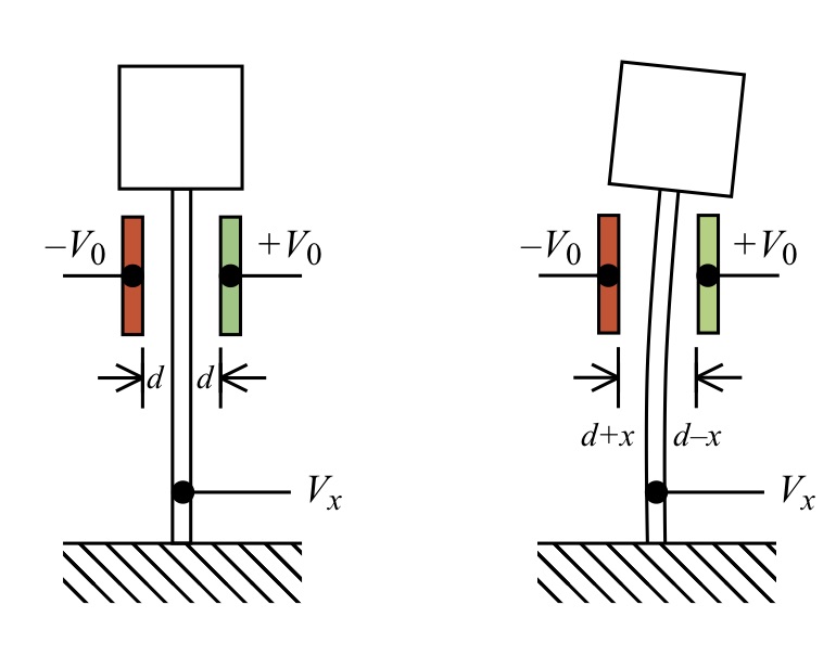
Fig. 14: Idealized accelerometer with applied voltage V_o.

From high school physics, the capacitance of a parallel plate is

where Q is the charge, V is the voltage, A is the plate’s area, and epsilon is the electrical permittivity of the gap. The two capacitors in Fig. 16 have capacitances C₁ and C₂, and charges Q₁ and Q₂, respectively. Conservation of charge requires

In terms of our two parallel plate capacitors,

Substituting for the capacitances in terms of the plate spacing yields

Canceling common terms and solving for the displacement x,

We showed above that the displacement x can be expressed in terms of the applied acceleration, mass, and beam stiffness. Substituting for x then gives our electro-mechanical governing equation that relates the acceleration a to the known quantities of beam stiffness k, mass m, nominal gap spacing d, and applied voltage V₀:

Consequently, the acceleration is linearly proportional to the induced voltage V_x, which can be measured. QED

APPENDIX B: GRAVITY IS AN ACCELERATION

Rather than delve into general relativity to demonstrate that gravity is an acceleration – for which I don’t have the necessary mathematical background in topology or group theory anyway! – we’ll use an intuitive argument to show that this is so. Consider a version of Einstein’s “elevator experiment” depicted in Fig. 15. In the figure^[4] an observer holding a ball is enclosed in a small room. In the first case the small room sits inside a rocket that is accelerating at 1g (9.8 m/s²) in outer space. In the other case the small room sits on the surface of the Earth. In both cases the observer drops a red ball. Based on the trajectory of the ball, it is impossible to decide whether the room is at rest in a gravitational field of 1g, or in space aboard a rocket that is accelerating at a rate of 1g. Consequently, one understands that gravity is an acceleration.

Fig. 15.

You needn’t journey to outer space to have experienced this equivalence between gravity and acceleration. If you’ve ever stood in an elevator car at rest your feet bear the weight of your body in the Earth’s gravitational field. This weight is the force due to gravity acting on your body’s mass: F = mg, where the force F here equals your weight, m is your mass, and g is the acceleration of gravity. If the elevator accelerates upward, the “weight” supported by your feet increases to F = m(g + a), where a is the elevator’s acceleration. You can feel your apparent weight increase until the elevator reaches a steady speed, e.g. it is no longer accelerating, at which point you feel only your own weight. And when the elevator decelerates you feel lighter since the car’s deceleration acts in opposition to the acceleration of gravity – which always points toward the Earth – so now F = m(g – a) where a is now a deceleration (hence the sign change). QED

v1.0

© copyright 2019, Shawn Burke, all rights reserved.  See Terms of Use for more info.

1. Personally, I’m not convinced. For now. As we saw in Part 1, hull speed is proportional to the cube root of the power you can get “into the water.” My opinion at the moment is that cadence is a secondary parameter, a byproduct of particular stroke mechanics. I’ve seen two paddlers win C1 Pro at the annual General Clinton 70-miler that had radically different strokes: One employed a long, slower, powerful stroke, while the other looked like they were beating eggs because their stroke was so fast. Maybe I’ll dig into the details in an article to come. ↑
2. https://www.dcrainmaker.com/2019/04/garmin-speed-cadence-sensors-v2-with-ant-bluetooth-smart-in-depth-review.html ↑
3. Hey, it’s wood: the original carbon fiber! ↑
4. Nice hat! ↑