by Shawn Burke, Ph.D.
OVERVIEW
An overview of canoe / kayak roll stability is presented. A qualitative model of free surface effect is introduced to investigate the influence of a partially swamped hull on roll angle.
INTRODUCTION
So, ever wonder why your hull flips? Yeah; me too. Usually after I’m home, dried off, and warming up under an afghan.
The obvious answer to “Why does a hull flip?” is that you heeled it too far. But what is “too far”? Why do hulls have roll stability in the first place? Why are some hull shapes more stable than others? And, why are some hulls “twitchy”?
Each of these questions has an answer, and not surprisingly the answers are based in physics. In this installment of the Science of Paddling series we’ll consider the problem of roll stability in general terms. Why general? Because hulls are so different. An Old Town Tripper canoe feels a lot different than an ICF kayak; they have radically different stability characteristics. A more detailed analysis requires hydrostatic models that are hull specific. You’ll also need naval architecture design and analysis software.
Rather than do a deep dive for each and every hull that might be of interest we’ll instead look at simplified models to provide insight into the questions above. And we’ll take a first look at the problem of free surface effect, or what happens when you partially swamp.
Our story begins more than 2,000 years ago, with an engineer named Archimedes.
OF HULLS AND RESTORING FORCES
There is an apocryphal tale of Archimedes running naked down the streets of Syracuse yelling “Eureka!” after having discovered a method for determining whether a golden crown was actually made of gold. The method relied on water displacement to determine the crown’s volume, a scale to determine its weight, and calculating its density from the ratio of weight to volume – then comparing that to the known density of gold. He supposedly figured out how to do this by observing the amount of water displaced in his bath after climbing in. Historians doubt that this ever happened; it doesn’t make sense from an engineering standpoint in light of the required precision for bathwater level measurement. But chilling out and taking a bath when inspiration hits does sound appealing.
Instead, in his treatise On Floating Bodies[1] this ancient Greek mathematician, scientist, philosopher, and engineer showed that an object floating in a liquid will displace a mass of liquid with weight equal to the that of the object. Once floating, the object continues to float; with all other factors constant it neither rises nor sinks after equilibrium is established. As we now know from Isaac Newton this equilibrium occurs because the there is a balance of forces, equal in magnitude and in opposite directions such that their sum equals zero. This is an embodiment of Newton’s First Law. The floating object’s weight “points” downward because of the acceleration due to gravity. The buoyancy force must have equal magnitude and “point” upward to satisfy equilibrium; the vectors cancel, not just their magnitudes. Turns out all that stuff about vectors in Part 18: Many Rivers to Cross are useful after all.
You are experiencing a balance of forces right in this moment – and you’re probably not aware of it. Your weight can be idealized as a vector acting through your center of mass (more on that in a moment), which means your weight – a force – has magnitude and direction. The direction is of course downward, toward the center of the Earth.[2] If your weight vector pointed up you’d float away; if it pointed sideways you’d accelerate right off the couch and into the cat, a wall, or whatever other object stands in your way. Unbalanced forces act to accelerate masses.
Since your weight vector points downward, and we know that you aren’t accelerating through the couch into the basement, from Newton we know there must be an equal and opposite force to satisfy static equilibrium. What is it? Well, strange as it may sound, your couch (or chair, or whatever you’re sitting or perhaps standing on as you read this) is applying this balancing force[3]. If you follow the chain of forces then a similar equilibrium exists between your chair or couch and the floor. Then between your house and its foundation upon the Earth.
As to where these force vectors act, an object with mass distributed over space can be idealized as a so-called “point mass” of zero dimension located at the object’s center of mass. Simply put, the center of mass is the location where you can apply a force to accelerate the object without causing it to rotate. Bear in mind that a point mass is merely a concept. It’s useful in representing the static and dynamics properties of an object without need to account for what happens to each of its parts.[4]
The location of your body’s center of mass will vary depending on how your various parts are arranged. We’ll assume that you’re arranged symmetrically side-to-side. As shown in Fig. 1, my wooden stunt double has a center of mass in the sagittal plane located below its naval when in a standing posture, and located near its solar plexus when in a seated posture; these are the locations where the figure is balanced on the tip of my finger. The stunt double doesn’t rotate and fall off my fingertip because the weight vector through its center of mass and the restoring force exerted by my finger are aligned.
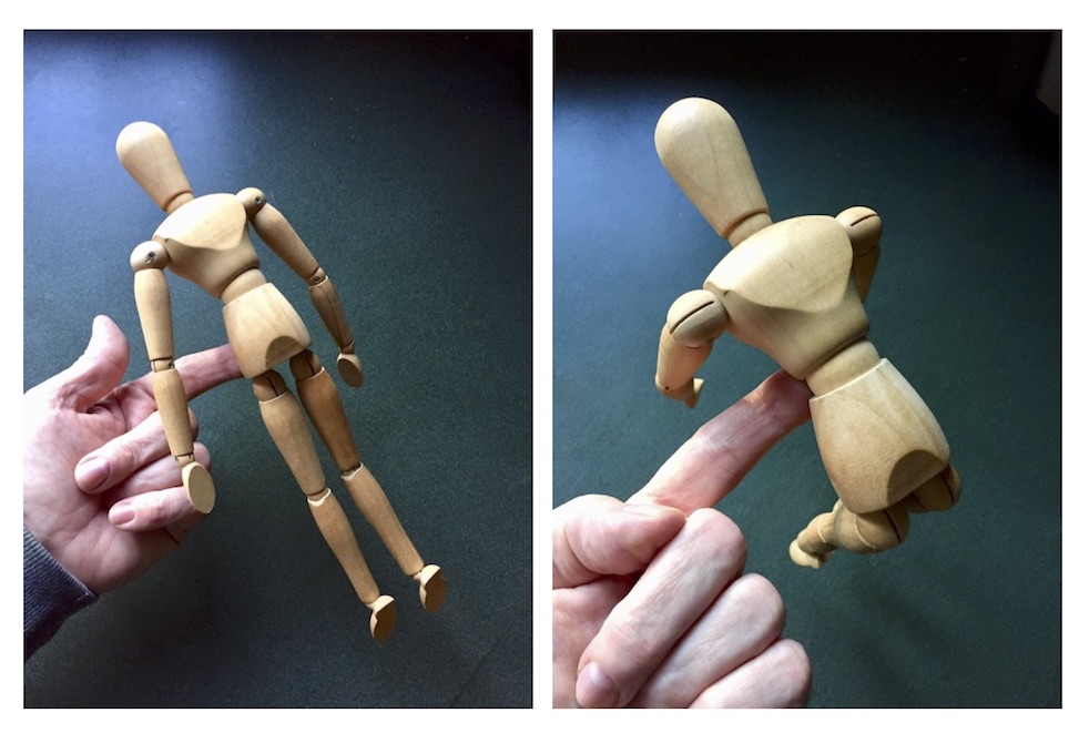
Figure 1: The body’s center of mass for two postures.
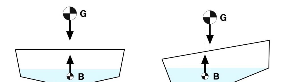
For floating objects, Archimedes posited that the buoyancy force acted upward – it is after all a buoyant force, not a sinking force – and can be idealized as acting through the center of mass of the displaced “hole” created in the water by the object. Let’s consider a specific example: a cylindrical log floating in the water. As shown in Fig. 2 the log displaces a certain volume of water. The weight of the displaced water equals the weight of the log. And the buoyant force acts upward, opposite to the log’s weight vector, and through the center of mass of the “hole” in the water created by the log. This location is called the center of buoyancy, and is labeled as B. Note that in Fig. 2 we aren’t asserting that the water has somehow seeped into the log as shown in the right-hand side of the drawing. Fig. 2 only suggests the equivalence of these two scenarios as long as the “virtual water” in the right-hand side drawing has “negative” weight, e.g. an upward pointing force vector. It makes the analysis easier.
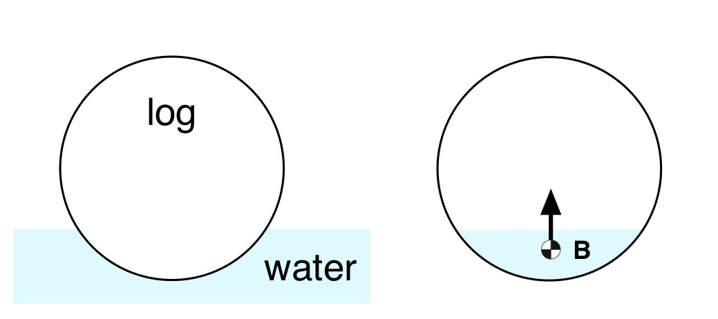
Figure 2: Log in water, and buoyant force location.
Let’s make things more interesting by putting an idealized paddler in an idealized hull with a semi-circular cross section. This scenario is depicted in Fig. 3.
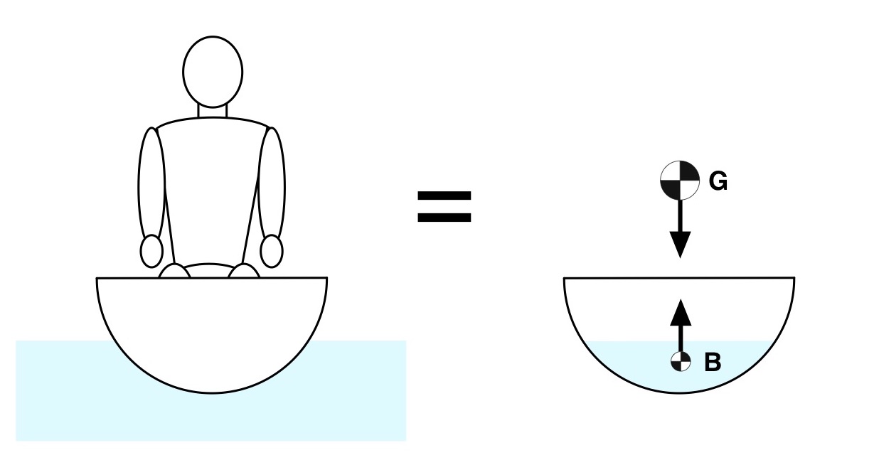
Figure 3: Paddler in hull with semi-circular cross section.
The center of mass G (sometimes called the center of gravity) is the location at which the combination of hull, paddler(s), and gear can be represented as a single point mass. Their combined weight is represented as a single downward-pointing weight vector acting through G. As suggested in the right-hand side of Fig. 3 the weight vector and the buoyancy force vector are aligned and cancel each other out. Since there are no unbalanced forces the hull and paddler will remain upright and floating.
But for anyone who’s paddled a hull like this, it gets a lot more interesting when you heel the boat – as if just climbing into that hull and trying to keep it vertical weren’t exciting enough. Heeling is shown in Fig. 4, using only point masses for clarity. When the circular hull heels the displaced volume of water keeps the same shape and position: a circular segment subtended by the hull’s surface and a chord at the waterline. As a result, the location of the center of buoyancy B for the circular hull never moves side-to-side. By contrast the center of mass of the hull plus paddler moves toward the heeled side. This results in unbalanced forces. And as we know from Newton, unbalanced forces accelerate masses. Which for our paddler means the hull will spin, the spin will accelerate, and unless they brace it’s trout scouting time.
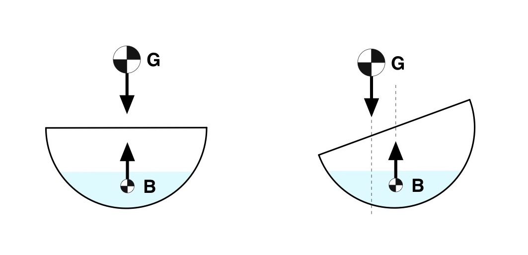
Figure 4: Semi-circular hull, vertical (left) and heeled (right).
For comparison, consider the V-bottomed, hard-chined hull depicted in Fig. 5. It looks a little bit like a 3×27 Pro Boat. Again, the hull and paddler can be idealized as a point mass located at the center of mass G, along with a balancing buoyant force at B. When the hull is vertical the respective force vectors cancel each other out, the hull floats, and everyone’s happy.
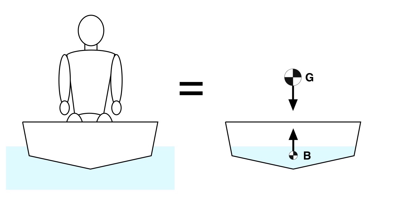
Figure 5: “Pro Boat” and point mass equivalents.
When this hull heels, the center of mass G moves toward the heeled side as before. But because of the hull’s cross-sectional shape something interesting happens with the center of buoyancy: it moves toward the heeled side, as depicted in Fig. 6.
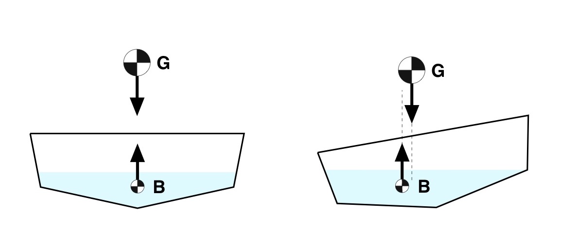
Figure 6: “Pro Boat” vertical and heeled.
Again, the forces are unbalanced and there is a net moment acting on the hull. But this time the buoyant force is outside of the weight vector. As a result, the moment created by the unbalanced forces will rotate the hull away from the heeled side rather than toward it. In this case the buoyant force acts as a restoring force. Then, as the hull rights itself the buoyant force moves back toward the keel line, always staying outside the weight vector until they’re aligned at the vertical. Because the hull is symmetric side-to-side, if the hull overshoots vertical the buoyant force will move toward the other side, staying outside the weight vector and thus righting the hull.
Now we’ve all flipped a hull or two. You can feel the restoring force help the hull set up at a certain lean angle and stay there. After this point, especially for racing hulls or highly elliptical hulls, the restoring force moves inside of your weight vector and you either brace or swim. The reason hulls do this is because after a certain heel angle you either put the gunnels below the waterline and swamp, or the center of buoyancy can no longer move outside of the center of mass at higher angles of heel.
This restriction on the center of buoyancy arises due to the shape of the hull. Because the hull sides curve upward, the shape of the subtended mass of water stops changing all that much after a certain heel angle. And since the buoyant force acts through the center of mass of this “hole” in the water, and its shape doesn’t change (much), the side-to-side location of B stops changing all that much with angle. And voila! Trout scouting. G has moved outside of B.
You can counter this tendency by extending a V-hull’s cross-section to infinity, and never introduce a chine. But infinitely wide boats don’t exist. Or, you could install an outrigger, which acts as a dependable restoring force – at least to the side with the ama! Or you could install sponsons, which you’ll find (for example) on Sportspal canoes. Or you can learn how to throw a brace.
One other thing about the relation between G and B: it’s better to be short. In Fig. 7 the center of masses for two paddlers of different heights are shown; the difference is exaggerated so that you can more easily see the difference. For a given angle of heel the taller paddler’s center of mass, and thus weight vector, are closer to the center of buoyancy than the short paddler’s center of mass. The taller paddler is closer to the stability limit. There is more margin for the shorter paddler, meaning the hull can heel further before they exceed the stability limit.
![]()
Figure 7: Movement of G for two paddler heights.
The cross-sectional shape of the canoe below the waterline also influences how the canoe “feels” about the vertical. A shallow arch hull will have a center of buoyancy that moves smoothly with heel, and the buoyancy vector’s intersection with the vertical line of the hull (a line passing through the keel and the center of mass) – the so-called metacentric height – is located well above G. A V-hull will have a center of buoyancy that moves abruptly with heel, and this intersection point travels rapidly down the hull line from the moment the hull is first heeled. Both hulls may eventually set up nicely after a certain amount of lean. But because B initially moves abruptly in a V-hull, and the metacentric height moves abruptly toward G, it will tend to feel “twitchy” about the vertical. Because… physics.
A SIMPLE MODEL OF ROLL
Note that in roll the hull plus paddler(s) experiences an exchange of kinetic and potential energies. This is because you have to do work in order to cause a hull to heel over, moving the center of mass G with respect to the waterline, and by lowering the center of buoyancy, or both. The buoyancy acts as a restoring force to move the hull back to its vertical equilibrium. Whenever I hear “restoring force” I think of springs. When the hull is heeled you can idealize potential energy being stored in a “buoyancy spring.” This potential energy is converted to kinetic (motion) energy as the hull rolls back to vertical.
This exchange of energies reflects how the hull has a natural rolling frequency, or time constant (the inverse of natural frequency). Since there are losses in the system the hull and paddler(s) don’t oscillate wildly; they tend to overshoot top dead center a bit before returning to vertical. This energy loss is a form of damping, analogous to resistance in electrical circuits for all the EEs out there.
In essence, the angle of the hull behaves like the angle of a pendulum over time. A simplified model is shown in Fig. 8, where the force due to gravity g, e.g. the weight of the pendulum, “rights” the pendulum to its resting position at the bottom of the arc. This “restoring force” has potential energy equal to the height the mass m is raised above its resting position times the weight of the mass (e.g., height times mg). Potential energy is exchanged for kinetic when the mass is released, and the pendulum swings – a model of how the hull rolls.
![]()
Figure 8: Pendulum model.
If you introduce viscous damping proportional to the angular rate at the pendulum’s hinge you can develop a qualitative model for how the angle of the hull plus paddler varies over time subject to external inputs, or to initial states of roll. Fig. 9 is a plot of the time varying angle of a simulated (and very simplified model of a) hull in roll. The initial state at time = 0 is a 11.46-degree heel.[5] Note how the hull slightly overshoots vertical, then asymptotically nulls out to a zero angle.[6] The time constant is set by the various parameters of the model which were chosen to give a generally representative response based upon experience; it does not correspond to the dynamics of any particular hull. No system identification[7] was undertaken.
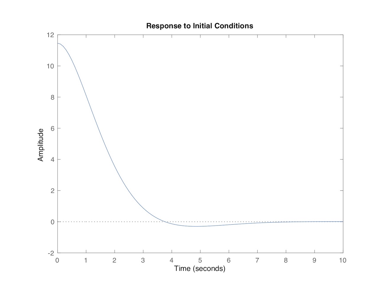
Figure 9: Hull roll angle (degrees) vs. time for simplified model.
We’ll visit the details of this model a bit later in the article.[8] In the process we’ll look at so-called free surface effects.
FREE SURFACE EFFECTS
If you paddle whitewater you’ve run at least a few rivers partially swamped. Waves lap over the gunnels, you’re busy negotiating a rock garden, and over time that slop over the sides adds up. In addition to the mass of the canoe, gear, and paddler there is now a slug of water with a mind of its own slithering around the bottom of your hull. It moves seemingly independent of the hull, and sometimes makes you pull a brace depending on the timing between the bilge water’s motion and the hull’s roll. They’re often out of phase, or partially out of phase.
By itself free surface effect doesn’t necessarily cause a hull to flip. External forces acting on a partially swamped hull do: more waves slapping against the coupled hull / water system, or paddlers having a hard time figuring out what the hull is doing in roll and placing poorly-timed strokes and braces. The combined hull / water system behaves differently.
Is it possible to simulate this coupling between hull and bilge water and gain some insight into the free surface effect? What follows is a first sketch toward modelling it. Note the key phrase “first sketch.” In a later article I’d like to revisit this model and add the effects from waves (a forcing function) and introduce a feedback loop model of the paddler (like a PID[9] controller) reacting to the hulls roll. Maybe update the parameters after figuring out a way of doing system identification. Future fun. But in the meantime…
Recall that we used a pendulum as a simple model for a hull in roll. This was motivated by how a floating hull experiences an energy exchange in roll between potential and kinetic energy, and the buoyancy force acts as a restoring force that brings the hull back toward vertical equilibrium. A slug of water in the bottom of a hull is just another mass. With a center of mass. And because the hull is floating (at least for the moment) there must be an added buoyancy force to compensate for the slug of water’s added weight. In essence this bilge water acts like the hull (e.g. a moving mass with a centroid that subtends an arc), which means a simple model for it is another pendulum. Since the water oscillates side-to-side at a different rate than the hull this second pendulum will have a different mass and length than the pendulum modeling the hull. Hmmm…
The remaining question is, how does the bilge water couple to the hull? In other words, can we come up with a simple way of modeling how the motion of the bilge water influences the motion of the hull, and vice versa? Those of you who’ve taken a sophomore linear systems course are probably yelling “Add a coupling spring!” at your screen right now. So I’ll take your advice and do just that.
Fig. 10 depicts a coupled double pendulum model for the combined hull / bilge water system. As before the hull is modeled by a first pendulum – the bits with the subscript ‘1’. The oscillating bilge water is modeled by a second pendulum – the bits with the subscript ‘2’. These two pendulums (aka, “pendula,” my new favorite word) are coupled via a linear spring with spring stiffness k. We’ll also add viscous damping proportional to the angular rate at the hinge points of the two pendula; this is not shown explicitly in the figure.
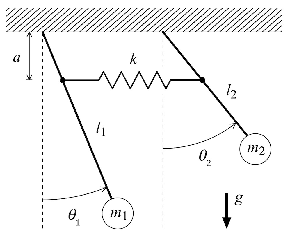
Figure 10: Coupled double pendulums.
The mathematical model for this system is derived in Appendix 1; check it out if you want to have even more fun. A corresponding Matlab simulation model is presented in Appendix 2, including the function which computes the A matrix (part of the state space model used by Matlab) for the coupled pendula. The parameters used in this model are presented in Appendix 2 as well; note that everything is in mks units.
So what happens? I looked at two scenarios, both simulating a hull initially heeled to 11.46 degrees, held steady there so the hull and water are not moving, then released. This is called a response to initial conditions. The combined weight of hull plus paddler is assumed to be 80kg. In the first scenario the mass of water is also 80kg. The time-varying angular response of the hull and water (modeled as pendula) for this case is plotted in Fig. 11.[10] The top plot is for the hull, while the bottom is for the water. The abscissa is time in seconds, while the ordinate is angle in degrees. Compare the top trace in Fig. 11 with the response of the empty hull plotted in Fig. 9. The small slug of water has a faster period of oscillation than the hull. And the water couples to the hull’s rolling motion, which is most apparent in how the hull roll angle vs. time settles near the vertical (0 degrees).
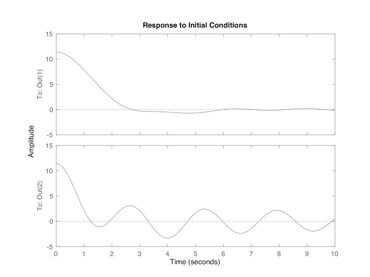
Figure 11: Coupled model with 80kg of water.
In the second scenario the mass of water is 400kg, or about 104 gallons; everything else is the same. The time-varying angular response of the hull and water for this case is plotted in Fig. 12. The top plot is for the hull, while the bottom is for the water. Compare the top trace in Fig. 12 with the response of the hull with 80kg of water plotted in Fig. 11. The larger slug of water has a slower period of oscillation than before, and a greater amplitude over time owing to its greater momentum. The water couples to the hull’s rolling motion to a greater degree, which is most apparent in how the hull roll angle vs. time settles near the vertical (0 degrees). Note that in this simplified model the spring constant used to model is the same for both simulations, as was the lever arm (‘a’ in Fig. 10) and second pendulum’s length. Rather than add even more assumptions about the model parameters I chose only to vary the mass of water between the two scenarios.
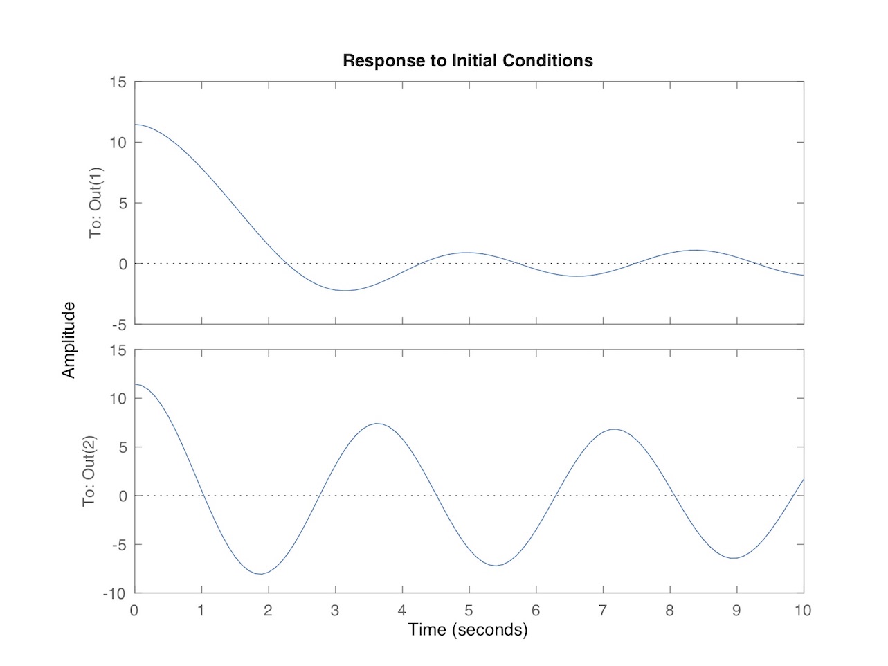
Figure 12: Coupled model with 400kg of water.
Since many of you will have questions about the model, and how varying the parameters change the simulation, I’ve included in Appendix 2 the source code listing for the Matlab function used to model the system, plus the parameters used in the model. I encourage you to work with it and have fun! If we can settle on what parameters are most representative of a real-world hull then there are many things we can investigate… in a future article.
SUMMARY
Phew! That was a long one, especially if you worked through the Appendices.
In this installment of the Science of Paddling we enjoyed (I hope) an overview of canoe / kayak roll stability. Buoyancy acts as a restoring force in roll. We saw that in the absence of external forces hulls flip when the center of buoyancy moves inside the hull plus paddler’s center of mass. It’s that simple.
A qualitative model of a hull plus paddler in roll was presented, along with a simple model of free surface effect coupling, to investigate the influence of a partially swamped hull on roll angle. By itself the free surface effect doesn’t necessarily cause the hull to flip. But experience suggests that external forces acting on a partially swamped hull – waves and the forces from paddling strokes – do. This will be worth investigating in a future article. Besides, who wouldn’t enjoy modeling a paddler as a feedback controller?
So for those of us who like running whitewater, we can now tell our friends why we flipped. “It was physics; not me!”
APPENDIX 1: Coupled Double Pendulum Model
Consider the double pendulum system depicted in Fig. 13 (yes, this is the same as Fig. 10, but it’s nice to have a copy close to the analysis). The two pendula have lengths l1 and l2, respectively, with end masses m1 and m2. There is a spring that couples the pendula with linear spring stiffness k, connected a distance a from their hinged bases. Each pendulum’s rotation is described by the angles q1 and q2. Not shown in the Figure is a viscous rotary damping about the hinges, modeled by the parameters b1 and b2. The first pendulum is a simple model of the combined hull and paddler in roll, while the second models the water sloshing about in the hull, as explained above.
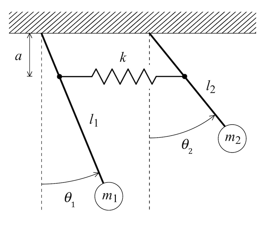
Figure 13: Coupled double pendulums.
We shall assume that the angles 


These are merely statements of Newton’s 2nd law for a two degree of freedom system. The left-hand side in each corresponds to the force from angular acceleration, while the terms on the right-hand side are forces acting in opposition to that acceleration: angular viscous damping, the restoring force due to gravity, and a spring force due to the its elongation or contraction. Note that in the absence of a spring (i.e., let the spring stiffness k go to zero) each pendulum has a separate governing equation in that there would be no
These equations can be simplified and written in the familiar homogeneous form of simple oscillators as


Defining


and adopting the time derivative notation

allows us to rewrite the governing equations in state space form
![\frac{d}{dt}\left[ \begin{matrix} {{\theta }_{1}} \\ {{{\dot{\theta }}}_{1}} \\ {{\theta }_{2}} \\ {{{\dot{\theta }}}_{2}} \\ \end{matrix} \right]=\left[ \begin{matrix} 0 & 1 & 0 & 0 \\ -{{\alpha }_{1}} & -{{\gamma }_{1}} & {{\beta }_{1}} & 0 \\ 0 & 0 & 0 & 1 \\ {{\beta }_{2}} & 0 & -{{\alpha }_{2}} & -{{\gamma }_{2}} \\ \end{matrix} \right]\left[ \begin{matrix} {{\theta }_{1}} \\ {{{\dot{\theta }}}_{1}} \\ {{\theta }_{2}} \\ {{{\dot{\theta }}}_{2}} \\ \end{matrix} \right]](https://s0.wp.com/latex.php?latex=%5Cfrac%7Bd%7D%7Bdt%7D%5Cleft%5B+%5Cbegin%7Bmatrix%7D++%7B%7B%5Ctheta+%7D_%7B1%7D%7D+%5C%5C++%7B%7B%7B%5Cdot%7B%5Ctheta+%7D%7D%7D_%7B1%7D%7D+%5C%5C++%7B%7B%5Ctheta+%7D_%7B2%7D%7D+%5C%5C++%7B%7B%7B%5Cdot%7B%5Ctheta+%7D%7D%7D_%7B2%7D%7D+%5C%5C++%5Cend%7Bmatrix%7D+%5Cright%5D%3D%5Cleft%5B+%5Cbegin%7Bmatrix%7D++0+%26+1+%26+0+%26+0+%5C%5C++-%7B%7B%5Calpha+%7D_%7B1%7D%7D+%26+-%7B%7B%5Cgamma+%7D_%7B1%7D%7D+%26+%7B%7B%5Cbeta+%7D_%7B1%7D%7D+%26+0+%5C%5C++0+%26+0+%26+0+%26+1+%5C%5C++%7B%7B%5Cbeta+%7D_%7B2%7D%7D+%26+0+%26+-%7B%7B%5Calpha+%7D_%7B2%7D%7D+%26+-%7B%7B%5Cgamma+%7D_%7B2%7D%7D+%5C%5C++%5Cend%7Bmatrix%7D+%5Cright%5D%5Cleft%5B+%5Cbegin%7Bmatrix%7D++%7B%7B%5Ctheta+%7D_%7B1%7D%7D+%5C%5C++%7B%7B%7B%5Cdot%7B%5Ctheta+%7D%7D%7D_%7B1%7D%7D+%5C%5C++%7B%7B%5Ctheta+%7D_%7B2%7D%7D+%5C%5C++%7B%7B%7B%5Cdot%7B%5Ctheta+%7D%7D%7D_%7B2%7D%7D+%5C%5C++%5Cend%7Bmatrix%7D+%5Cright%5D&bg=ffffff&fg=000&s=0&c=20201002)
This has the familiar form

which lends itself to simulation in modeling and analysis software packages such as Matlab.
Since Matlab requires a full state space representation, we’ll further define B, C, and D matrices such that


For scalar input u, and
![\mathbf{B}=\left[ \begin{matrix} 0 \\ 0 \\ 0 \\ 0 \\ \end{matrix} \right]](https://s0.wp.com/latex.php?latex=%5Cmathbf%7BB%7D%3D%5Cleft%5B+%5Cbegin%7Bmatrix%7D++0%C2%A0+%5C%5C++0%C2%A0+%5C%5C++0%C2%A0+%5C%5C++0%C2%A0+%5C%5C++%5Cend%7Bmatrix%7D+%5Cright%5D&bg=ffffff&fg=000&s=0&c=20201002)
![\mathbf{C}=\left[ \begin{matrix} 57.29577 & 0 & 0 & 0 \\ 0 & 0 & 57.29577 & 0 \\ \end{matrix} \right]](https://s0.wp.com/latex.php?latex=%5Cmathbf%7BC%7D%3D%5Cleft%5B+%5Cbegin%7Bmatrix%7D++57.29577+%26+0+%26+0+%26+0%C2%A0+%5C%5C++0+%26+0+%26+57.29577+%26+0%C2%A0+%5C%5C++%5Cend%7Bmatrix%7D+%5Cright%5D&bg=ffffff&fg=000&s=0&c=20201002)
![\mathbf{D}=\left[ \begin{matrix} 0 \\ 0 \\ \end{matrix} \right]](https://s0.wp.com/latex.php?latex=%5Cmathbf%7BD%7D%3D%5Cleft%5B+%5Cbegin%7Bmatrix%7D++0%C2%A0+%5C%5C++0%C2%A0+%5C%5C++%5Cend%7Bmatrix%7D+%5Cright%5D&bg=ffffff&fg=000&s=0&c=20201002)
The input matrix B is zero because we’re not including any exogenous inputs[11]. The matrix D is zero because we’re not including any feedthrough terms[12]. And the C matrix includes the numbers 57.29577 because angles in our model are expressed in radians, and we wish to represent angle outputs in the more familiar units of degrees.
Finally, to recover the simple single-pendulum model just set the value of the spring stiffness k to zero. This will decouple the two pendulums, so the double pendulum just becomes to completely independent single pendulum models. Pick one, and that’s your single pendulum.
APPENDIX 2: MATLAB Model
The function ‘couppend’ models the coupled pendulum given values for the gravitational constant g, pendulum lengths l1 and l2, point masses m1 and m2, damping coefficients b1 and b2, and lever arm a. It returns the A matrix for a state space model of the system.
Note angles and angular rates are modeled in radians and radians / second, respectively.
function amat = couppend(g,l1,l2,k,m1,m2,b1,b2, a)

alpha1 = g/l1 + (k/m1)*(a/l1)^2;

alpha2 = g/l2 + (k/m2)*(a/l2)^2;

beta1 = (k/m1)*(a/l1)^2;

beta2 = (k/m2)*(a/l2)^2;

gamma1 = b1/(m1*l1^2);

gamma2 = b2/(m2*l2^2);

amat = [0 1 0 0;-alpha1 -gamma1 beta1 0;0 0 0 1;beta2 0 -alpha2 -gamma2];

end
This returns the A matrix for a linear time invariant (LTI) state space model of the form
where we define B, C, and D matrices as
>> b=[0 0 0 0]';

>> c=[57.29577 0 0 0;0 0 57.29577 0];

>> d=[0;0]';
This B matrix signifies that there is no external input or modeled feedback control; the C matrix lets us display the angles over time in degrees (hence the 57.29577 rather than 1); the zero D matrix models feed-through (like in most noise-cancelling headphones) which here is zero.
After defining all four state space matrices, at the Matlab command window, enter (for example):
>> a=couppend(9.8,10,4,1000,80,80,12000,000,2);

>> canoeroll=ss(a,b,c,d);

>> initial(canoeroll,[.2 0 .2 0]’,10);
where 0.2 radian = 11.46 deg. The Matlab function ‘initial’ takes a matrix of ‘sys’ format then calculates and plots the response to initial conditions over the specified time interval. This particular call leads to the plot in Fig. 11 above.
v1.0
Copyright (c) 2020, Shawn Burke. All rights reserved. See Terms of Use for more info.
- https://archive.org/details/worksofarchimede00arch/page/262/mode/2up, pp. 263-300 ↑
- We’ll assume that you’re not floating weightless on the International Space Station. ↑
- Each is both cause for and effect from the other; give it some thought and you’ll come to the same conclusion. Those of you familiar with “dependent arising” are no doubt smiling. ↑
- For those with a philosophical bent this reflects science and engineering’s ability to tell us about what things do, but their silence about what they are. They are functional, not ontological. As Newton wrote with regard to his model of gravity, “I have not as yet been able to discover the reason for these properties of gravity from phenomena, and I frame no hypotheses.” (“hypotheses non fingo”) ↑
- 11.46 degrees is 0.2 radians, a convenient number to use in the simulation. ↑
- Since this is a linear time invariant (LTI) model it theoretically takes an infinite amount of time to actually reach zero. If you include nonlinear damping you can make the angle null out in a finite amount of time. But since this is already a hand-wavy model, why make it even more hand-wavy by assuming a particular nonlinear damping model; which one would you choose, and why? ↑
- SysID is a process well known to control systems engineers where responses to known inputs are measured and used to construct a high-fidelity model of an actual system. ↑
- And yes, the restoring force on a hull acts like a hardening (then abruptly softening) spring as the hull first heels, then capsizes. Modeling this would be hull-specific and beyond what we’re looking to do here: develop insight without undue complication. So we use a linear spring model. Your mileage may vary. ↑
- Proportional-Integrator-Differentiator – PID is the acronym for simple single input / single output (SISO) controllers. ↑
- Note that there are a lot of assumptions inherent in the model, so try not to interpret these results too literally! ↑
- Like waves slapping against the hull, or righting moments exerted by the paddler. The latter effect would be interesting to model – someday – using a feedback loop with a regulator. ↑
- Feedthrough terms are the bane of many control system designers. Yet feedthrough is how most noise canceling headphones work, injecting “anti-noise” to cancel out noise at the ear. ↑