by Shawn Burke, Ph.D.
SUMMARY
In this installment of The Science of Paddling we’ll take a look at how things don’t always work out when writing these articles. Or when doing engineering analysis in general. Sometimes blind spots let us take long and fascinating trips to nowhere. Like thinking we’ve “solved” the paddling power measurement problem. Along the way we’ll re-introduce Newton’s Laws of Motion and review inertial frames of reference.
INTRODUCTION
One thing you don’t see enough in the science and engineering literature is articles about why or when things don’t work out – and I’m not talking about catastrophic failures like the Tacoma Narrows Bridge. To the uninitiated each new press release or publication fairly teems with breathless tales of world-changing achievement, offering glimpses into a Potemkin reality consisting only of 100% inspiration and success, and 0% perspiration, let alone any hint of dead ends or (eek!) failure.
Now “bolts out of the blue” do sometimes occur that lead to surprising if not even significant results. I drafted the entirety of my Master’s thesis in a single weekend while I was ostensibly visiting my girlfriend; the insight of how to untangle what had been an intractable mess of equations – and months of dead ends – revealed itself on the drive to see her. But those moments are rare and precious. As are weekends with your girlfriend![1]
Instead, the process underlying most science and engineering R&D is generally characterized by 10% inspiration and 90% perspiration, along with a lot of dead ends entailing work that leads to no usable result. The hope is that, no matter what, you learn something useful along the way that prepares you for the next adventure.
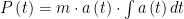
In case you’re wondering, yes, there are a lot of chicken scratchings, simulations, and data explorations that ended up on the proverbial cutting room floor as I’ve written these articles. An example, and the basis for the first half of this article, appears in Fig. 1. What actually gets posted are the analyses that survive revision and scrutiny.
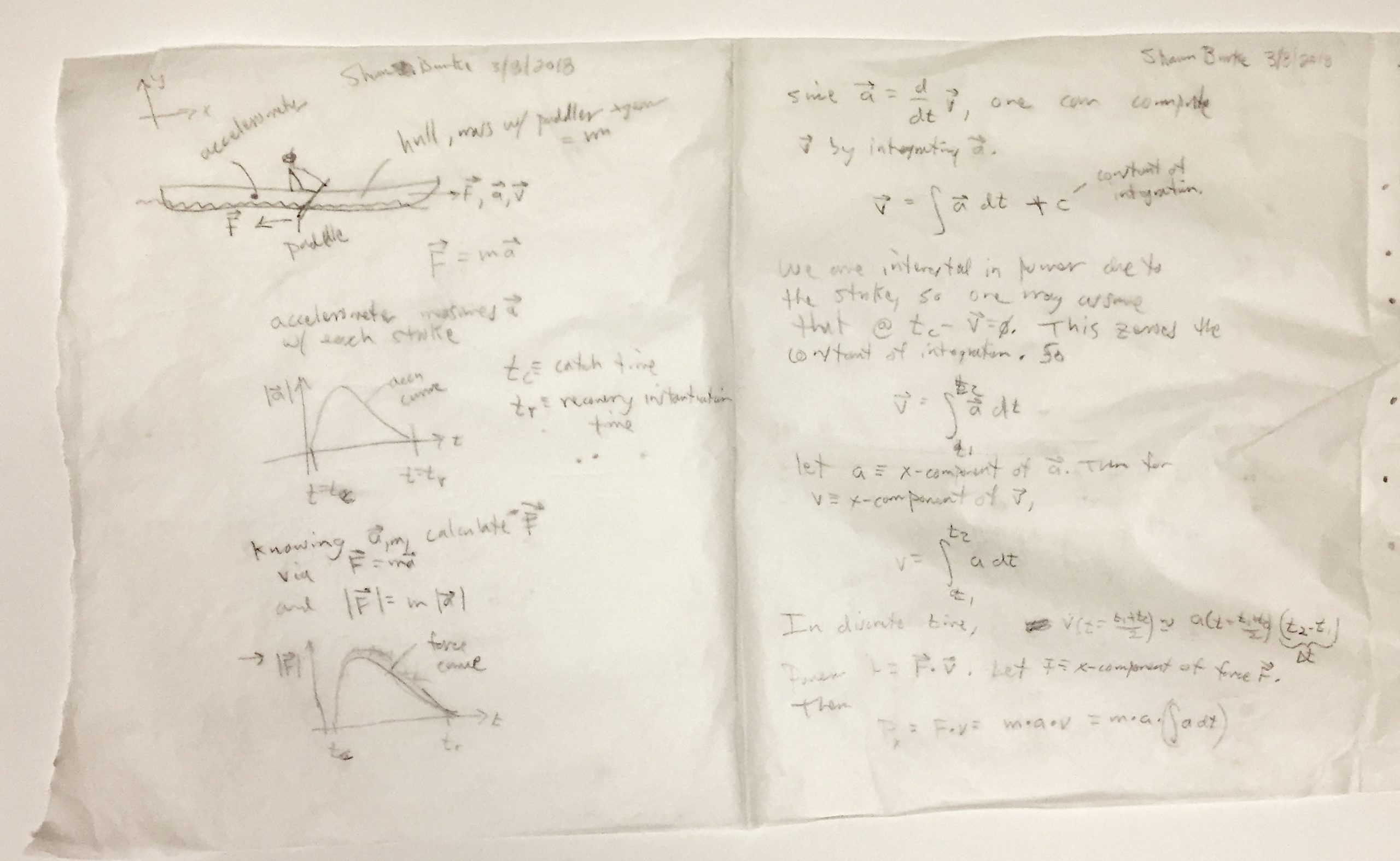
Figure 1: Equations ‘n stuff.[2]
So in this installment in the Science of Paddling Series we’ll take a look at one of my adventures down the rabbit hole in pursuit of a simple way to measure paddling force, and paddling power. Just know before we start that what I propose won’t work; in fact, physics demonstrates that in general it can’t. We’ll start by making some bad assumptions.
WHAT IS FORCE?
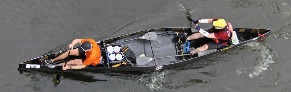
Consider the C-1 paddler depicted in Fig. 2. As they paddle a force is exerted through the blade via the shaft, directed toward the stern.
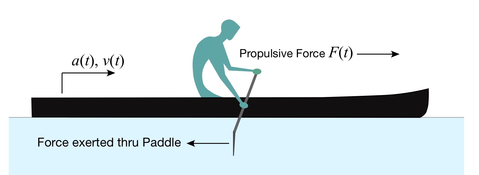
Figure 2: C-1 Paddler.
Newton’s Third Law of Motion states:
“To every action there is always opposed an equal reaction: or the mutual actions of two bodies upon each other are always equal, and directed to contrary parts.”
Here, “action” means force. Since there is a paddle force exerted in one direction, there must be an equal force (the reaction) “directed to contrary parts,” e.g., in the opposite direction of the paddle force. We’ll call this the propulsive force F(t).
Newton’s First Law of Motion states:
“Every body persists in its state of being at rest or of moving uniformly straight forward, except insofar as it is compelled to change its state by force impress’d.”
In other words, the hull is stationary until you exert a paddle force, e.g. “compel” the canoe to “change its state by force impressed.” Further, if the hull is already moving at a steady speed – its “state… of moving” – in order to make it move faster you must apply a suitable propulsive force. The canoe’s state is represented, for example, by a velocity v(t) in the direction of the propulsive force.[3] This should be familiar to all of you; we’re just reviewing it in order to motivate and support the ensuing analysis.
Finally, Newton’s Second Law of Motion states:
“The alteration of motion is ever proportional to the motive force impress’d; and is made in the direction of the right line in which that force is impress’d.”
This means in the present case that changes in velocity are proportional to the propulsive force, and those changes occur in the same direction as that force.
All of these Laws of Motion appeared in Newton’s Mathematical Principals of Natural Philosophy, published in 1687. In order to make the Second Law more tangible you have to dive into this text a bit, whereupon you learn that the “alteration of motion” recited in the Law is actually the time rate of change of an object’s momentum. That is,
![F\left( t \right)=\frac{d}{dt}\left[ mv\left( t \right) \right]](https://s0.wp.com/latex.php?latex=F%5Cleft%28+t+%5Cright%29%3D%5Cfrac%7Bd%7D%7Bdt%7D%5Cleft%5B+mv%5Cleft%28+t+%5Cright%29+%5Cright%5D&bg=ffffff&fg=000&s=0&c=20201002)
where m is the combined mass of hull and paddler. Recall from Part 5: What Moves You that momentum is the product of mass and velocity. Newton would have referred to the right-hand side of this equation as a fluxion, indicating a rate of change with respect to time of the quantity in brackets[4]. We now call it a derivative; here, the derivative of momentum with respect to time.
Since our hull and paddler have constant mass[5] this equation takes on the familiar form
![F\left( t \right)=m\frac{d}{dt}\left[ v\left( t \right) \right]=ma\left( t \right)](https://s0.wp.com/latex.php?latex=F%5Cleft%28+t+%5Cright%29%3Dm%5Cfrac%7Bd%7D%7Bdt%7D%5Cleft%5B+v%5Cleft%28+t+%5Cright%29+%5Cright%5D%3Dma%5Cleft%28+t+%5Cright%29&bg=ffffff&fg=000&s=0&c=20201002)
where a(t) is the hull’s acceleration.
In looking at this equation a thought came to mind. To measure the paddle force directly one must place sensors on the paddle, along with signal conditioning electronics, a power source, and most likely a radio transmitter to send the sensor signals to either a data recorder, a smart phone app, or the like. But Newton’s Third Law states that this force must equal the propulsive force. (Note that this is my first mistake, but bear with me.) And equation (24.2) states that if I know the combined mass of the hull and paddler – which can be determined very simply by just using a scale – then measure the acceleration of the hull in the direction of travel while paddling, you can calculate the propulsive force, which then equals the paddle force! (Note that this inference, being based upon mistaken prior assumptions, is also wrong; but bear with me.)
Woo hoo!
The propulsive force curve, as we saw in Part 11: About the Bend, resembles a portion of a phase-shifted cosine function, as shown in Fig. 3.
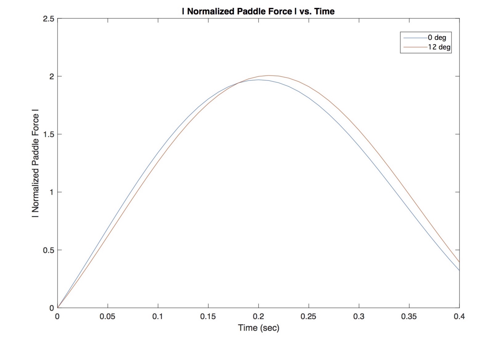
Fig. 3: Normalized paddle force vs. time.
Since the mass is constant, one can assume that the propulsive force will have the same general character. Further, there are smart phone apps that use the accelerometer built in to most modern smart phones to measure acceleration[6], and record this data to a file for later analysis in Matlab or similar software packages. So all I had to do was download an app to my smartphone, secure the phone in the bottom of my hull, and record data. It sounded almost too easy! Fortunately it was March 3rd, and the rivers near me were still frozen, and I didn’t. But I get ahead of myself…
TALES OF POWER,[7] PART 1
If you can compute paddling force, and have access to velocity data, you can calculate paddling power. This is because power is the product of force and velocity, as we discussed in Part 1: Tandem vs Solo, and in Part 9: Power to the Paddlers. Since we already have acceleration data from the smart phone’s accelerometer, and know that acceleration is the time derivative of velocity, then we can employ the inverse operation of taking a derivative, known in many intro calculus courses as an “anti-derivative” or more commonly as an integral, to compute velocity via

The elongated ‘S’ indicates an integral, while the ‘dt’ shows that this operation is an integral over time. Power can then be expressed rather simply (and incorrectly, but bear with me) as
Since there is no propulsive paddle force when the paddle is out of the water, from its removal at the initiation of recovery until the moment of catch, the average power over a stroke is
![{{P}_{avg}}=\frac{m}{{{t}_{1}}-{{t}_{2}}}\cdot \int\limits_{{{t}_{0}}}^{{{t}_{1}}}{\left[ a\left( t \right)\cdot \int{a\left( t \right)dt} \right]dt}](https://s0.wp.com/latex.php?latex=%7B%7BP%7D_%7Bavg%7D%7D%3D%5Cfrac%7Bm%7D%7B%7B%7Bt%7D_%7B1%7D%7D-%7B%7Bt%7D_%7B2%7D%7D%7D%5Ccdot+%5Cint%5Climits_%7B%7B%7Bt%7D_%7B0%7D%7D%7D%5E%7B%7B%7Bt%7D_%7B1%7D%7D%7D%7B%5Cleft%5B+a%5Cleft%28+t+%5Cright%29%5Ccdot+%5Cint%7Ba%5Cleft%28+t+%5Cright%29dt%7D+%5Cright%5Ddt%7D&bg=ffffff&fg=000&s=0&c=20201002)
The limits of integration t0 and t1, e.g. the range of times over which you perform this anti-derivative, correspond to the stroke’s catch and recovery initiation, respectively, for example as the times ‘0’ and ‘0.4’ in the normalized force curve plot Fig. 3. This is the stroke’s power phase (no pun intended). There are some subtleties to this calculation, such as how one deals with the constants of integration, as well as how to automatically detect when in time the catch and recovery initiation have actually occurred. But I’d encountered these complications before and so wasn’t worried.
Looks great, doesn’t it? Drop an accelerometer in the bottom of your hull, and voila! Paddle force and power are yours for the taking.
The problem is, it’s all wrong.
Take a look at Fig. 2. What’s missing? For those of you who read Part 14: Kind of a Drag you’ll recall that there is a third force acting here: the drag force. Newton’s First Law of Motion must incorporate all forces acting on an object, not just the ones you prefer; we’ll return to this point in a bit. This means Newton’s Second Law must be written as
![F\left( t \right)=m\frac{d}{dt}\left[ v\left( t \right) \right]+{{F}_{drag}}](https://s0.wp.com/latex.php?latex=F%5Cleft%28+t+%5Cright%29%3Dm%5Cfrac%7Bd%7D%7Bdt%7D%5Cleft%5B+v%5Cleft%28+t+%5Cright%29+%5Cright%5D%2B%7B%7BF%7D_%7Bdrag%7D%7D&bg=ffffff&fg=000&s=0&c=20201002)
As we learned in Part 14 the drag force acts in opposition to your motion; that’s why it on the opposite side of the equation from the propulsive force. It is also a property of the hull and its hydrodynamics. So in order to calculate the propulsive force you need to also measure the drag force. Turns out that making bad assumptions comes back to bite you in light of a correct application of physics. It’s actually embarrassing. At least I came to my senses.
But wait; didn’t we come up with a way of measuring the drag force in Part 14? Is it possible to salvage some good analysis from this train wreck? Well read on and find out.
TALES OF POWER, PART 2
The basis for the first second half of this article appears in Fig. 4; at least a portion of it. The question is will this too survive the impartial yet exacting scrutiny of physics?
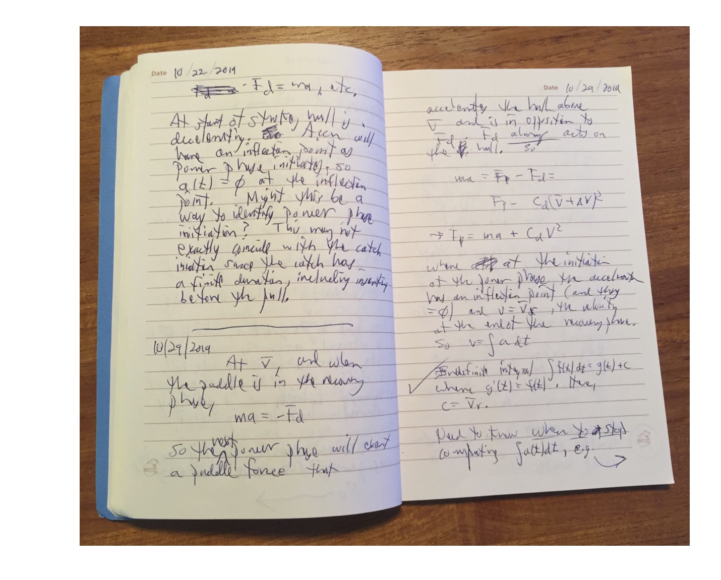
Figure 4: More nifty equations ‘n stuff.
Consider the C-1 paddler depicted in Fig. 5. We now incorporate all of the forces on the hull – we hope – because a careful reading of Newton’s Third Law of Motion indicates, “To every action there is always opposed an equal reaction” [emphasis added]. Every means, well, every, not just the actions (e.g., forces) you might be most interested in.
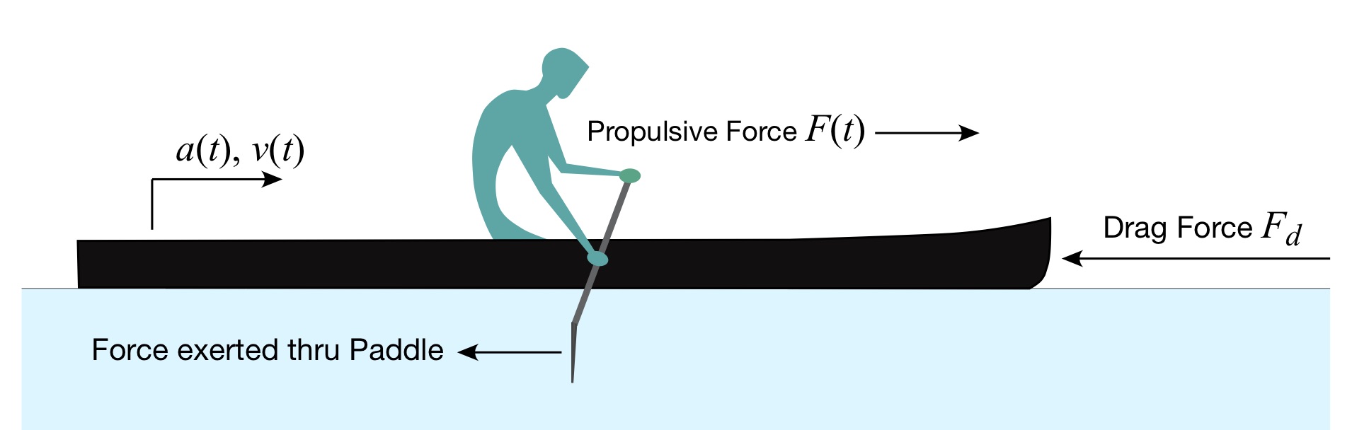
Fig. 5: C-1 Paddler with more forces.
Science of Paddling readers are of course familiar with the drag force. From Part 14: Kind of a Drag, we can represent the drag force Fdrag as proportional to the square of the hull’s velocity[8],
Where Cd is the drag coefficient. The drag coefficient is a constant, and as we learned in Part 14 can be measured via field tests. As a result, Equation (24.6) can be written as
![F\left( t \right)=ma\left( t \right)+{{C}_{d}}{{v}^{2}}\left( t \right)=ma\left( t \right)+{{C}_{d}}{{\left[ \int{a\left( t \right)dt} \right]}^{2}}](https://s0.wp.com/latex.php?latex=F%5Cleft%28+t+%5Cright%29%3Dma%5Cleft%28+t+%5Cright%29%2B%7B%7BC%7D_%7Bd%7D%7D%7B%7Bv%7D%5E%7B2%7D%7D%5Cleft%28+t+%5Cright%29%3Dma%5Cleft%28+t+%5Cright%29%2B%7B%7BC%7D_%7Bd%7D%7D%7B%7B%5Cleft%5B+%5Cint%7Ba%5Cleft%28+t+%5Cright%29dt%7D+%5Cright%5D%7D%5E%7B2%7D%7D&bg=ffffff&fg=000&s=0&c=20201002)
Then the power, which is the product of force and velocity, along with the velocity (which itself is the integral of acceleration), results in
![P\left( t \right)=\left\{ ma\left( t \right)+{{C}_{d}}{{\left[ \int{a\left( t \right)dt} \right]}^{2}} \right\}\int{a\left( t \right)dt}](https://s0.wp.com/latex.php?latex=P%5Cleft%28+t+%5Cright%29%3D%5Cleft%5C%7B+ma%5Cleft%28+t+%5Cright%29%2B%7B%7BC%7D_%7Bd%7D%7D%7B%7B%5Cleft%5B+%5Cint%7Ba%5Cleft%28+t+%5Cright%29dt%7D+%5Cright%5D%7D%5E%7B2%7D%7D+%5Cright%5C%7D%5Cint%7Ba%5Cleft%28+t+%5Cright%29dt%7D&bg=ffffff&fg=000&s=0&c=20201002)
and the average power over the stroke is
![P=\frac{1}{{{t}_{1}}-{{t}_{0}}}\int\limits_{{{t}_{0}}}^{{{t}_{1}}}{\left[ \left\{ ma\left( t \right)+{{C}_{d}}{{\left[ \int{a\left( t \right)dt} \right]}^{2}} \right\}\int{a\left( t \right)dt} \right]dt}](https://s0.wp.com/latex.php?latex=P%3D%5Cfrac%7B1%7D%7B%7B%7Bt%7D_%7B1%7D%7D-%7B%7Bt%7D_%7B0%7D%7D%7D%5Cint%5Climits_%7B%7B%7Bt%7D_%7B0%7D%7D%7D%5E%7B%7B%7Bt%7D_%7B1%7D%7D%7D%7B%5Cleft%5B+%5Cleft%5C%7B+ma%5Cleft%28+t+%5Cright%29%2B%7B%7BC%7D_%7Bd%7D%7D%7B%7B%5Cleft%5B+%5Cint%7Ba%5Cleft%28+t+%5Cright%29dt%7D+%5Cright%5D%7D%5E%7B2%7D%7D+%5Cright%5C%7D%5Cint%7Ba%5Cleft%28+t+%5Cright%29dt%7D+%5Cright%5Ddt%7D&bg=ffffff&fg=000&s=0&c=20201002)
Eureka! Paddling power from known or easily knowable parameters (combined mass of hull plus paddlers, and drag coefficient) plus a quantity that is measurable in real time (acceleration)!
Or so I thought. But something was niggling at me, and just wouldn’t stop. Can you see why this result is, in general not correct?
Hint 1: Total forces. All of them. Hint 2: Frames of reference.
You see, I’ve once again neglected all of the forces that can act on a hull. Let’s illustrate this with an update of Fig. 5:
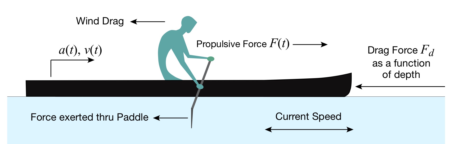
Figure 6: C-1 paddler with even more forces and effects.
Along with the various forces and state variables depicted in Fig. 6, this figure depicts the effect of wind, which may be a headwind, tailwind, or something in between. As we’ve all experienced, wind exerts a force that can be helpful or not – and can really mess with things if it kicks up big waves. Next, as we learned in Part 4: Shallow Water, and Part 20: Cutting Corners, there are depth-dependent effects that can impede us, and present themselves to the paddler as another drag force beyond form drag as the water gets shallow. In that way the drag coefficient is a function of depth; recall that we measured Cd in Part 14 in deep water. The combination of wind and depth-dependent drag forces means that we haven’t accounted for “every action,” as Newton pointed out we must do. So now we need a model of the drag coefficient vs. depth… as well as a depth meter to tell us which value of the drag coefficient to use at any moment (e.g., depth) in time. Plus we’ll need something to measure the wind and its direction, along with a 3-D model of wind drag for the hull and paddler. Needless to say, this is all sounding more than a little complex.
Next, current. You might ask yourself, why do I care? Let’s say I’m paddling in deep water with no wind; can’t I use the model derived above to infer paddling force and power from the acceleration measurement?
Let’s briefly return to the Appendix in Part 16: Cycles and Cycloids. Accelerometers make measurements with respect to a so-called “inertial frame of reference.” This means the accelerometer measures acceleration with respect to the Earth, which it considers to be fixed. Consequently, the in-hull acceleration measurements described above are referenced to the shoreline.
Why might this be a problem? Consider the following scenario[9]: Paddling upstream in a current that exactly equals your paddling speed. In this case you’re stationary with respect to the shore. As you paddle there will be some acceleration with respect to the shore frame of reference. But the velocity you compute by integrating the accelerometer signals will just be the increments of added speed during the stroke’s power phase, not your speed with respect to the current. And remember, the drag force is expressed in terms of your speed with respect to the hull’s movement relative to the water, not relative to the shoreline. Oops. Wrong velocity.
So can you fix this reference frame issue in general by, say, using a GPS receiver to calculate your locally-average velocity over ground (e.g., tied to the shore frame of reference), then use the accelerometer to compute the increments of velocity above this average velocity to deduce what’s happening during the power phase? Well, it might be possible. But doing so adds even more complication to what I had hoped might be a single, simple measurement. And it doesn’t address the role of any wind force in the “every action” constraint.
And that, is that. Well, at least it was a fun way to get “No” for an answer!
CONCLUSION
In their landmark paper, “Sound waves in rooms,” Philip Morse and Richard Bolt wrote of a need to “salt our analysis with liberal doses of common sense.” And that’s certainly the case here. It’s very, very easy to become enamored with our tools, and lose sight of what we’re actually trying to accomplish. And it’s often difficult to let go of something, even when its range of useful application becomes so small that it essentially vanishes.
As I look at the wall of engineering, mathematics, and science texts in front of me right now, I wonder at how it’s possible to keep “enough” of all that stuff in mind to accomplish, well, anything. A fellow engineer once asked if I was worried that a feedback control system I had designed might have a sign error or two buried in its parameters. My reply (which I have since deeply regretted) was, “We’ll find out when we turn it on.” He turned to face me, looked me in the eye, and noted, “Remind me not to fly in any spacecraft you design.” Needless to say, we simulated and tested the daylights out of that control system before integrating it into the final hardware. Control for all factors, and verify.
So in this installment of The Science of Paddling I hope you’ve come to appreciate the value of salting our analysis with liberal doses of common sense, all along the way. We’ve seen that to develop a meaningful (or even workable) engineering system all factors have to be accounted for. And if you choose to neglect them, only do so after first identifying all effects, then assessing their relevance and impact. You know; solid engineering practice ‘n stuff. The good news regarding the analysis presented here – at least for me – is I knew when to put fingers to keyboard, and when to not.
REFERENCES
P.M. Morse and R.H. Bolt, “Sound waves in rooms,” Reviews of Modern Physics, Vol. 16, pp. 69-150 (1944).
© 2020, Shawn Burke, all rights reserved. See Terms of Use for more information.
v1.0-B
-
For those of you who like happy endings, she and I have been married now for nearly 35 years. I think it helped that she too was an MIT student… ↑
-
Written on a continuous roll of shelf paper at a New York hotel. You never know when the need for analysis will hit! ↑
-
For those of you with a linear systems theory background the velocity is a so-called state variable; it represents a state of the system. ↑
-
The notation used here, however, is due to Leibniz, who developed calculus independently of Newton. ↑
-
A common example of a system whose mass is not constant is a rocket, which gets lighter as it ascends since its mass of fuel is consumed to generate thrust. ↑
-
These are solid-state MEMS accelerometers like the one we encountered in Part 16: Cycles and Cycloids. In phones they’re often used to determine the phone’s spatial orientation. ↑
-
Any Carlos Castaneda readers out there? ↑
-
This is true at racings speeds, although as noted in Part 14 there are other models that include linear as well as fractional power terms. But for the moment those details would take us too deep into the weeds and distract us from a much-needed 30,000-foot view. ↑
-
You can come up with other scenarios for extra credit! ↑