by Shawn Burke, PhD

Introduction

The best laid plans of mice and men go oft awry… I decided to write an article on wave surfing and wake riding. But then I realized that necessitates writing about how water waves propagate. That requires writing about the differences between dispersive and non-dispersive waves, shallow and deep water, and linear versus nonlinear waves. And since I’d never written about nonlinear surface waves, better cover that, too. That’s the trap we fall into with any reductionist system: an infinite regression. Or at least it seems like that.^[1]

So, in this installment of the Science of Paddling series we’ll review some general concepts about water waves, linear and nonlinear, as a prelude to wave surfing and wake riding. Along the way we’ll wade into a 19^th century scientific controversy about whether certain types of water waves actually exist. (Hint: they do.). I’ve walled off the more complex math in a section at the end called ‘Extra Credit’ for those who’d like to dive in a bit deeper.

To write this article I’ve drawn from my grad school course notes on acoustics, wave propagation, nonlinear wave propagation, and nonlinear partial differential equations, along with associated physics and mathematics texts. This all reminded me that the field of wave propagation is vast; we couldn’t cover it all in our lifetimes. What you’ll read here is more like a fireside chat, a distillation of relevant concepts that would help you in a Tuesday night pub quiz… if the pub happened to be on the campus of MIT.^[2]

Preliminaries

We begin by reviewing some general concepts from the theory of wave propagation: frequency, wavelength, velocity, and dispersion. We’ll draw from acoustics to explain dispersion in practical terms.

The relationship between a wave’s frequency f, period T, and angular frequency is defined by

(1)

Formally, we call f the circular frequency, although just ‘frequency’ usually suffices. It has units of cycles per second, or Hertz (‘Hz’).

The circular frequency is the rate of change of a sinusoidal waveform’s phase before the waveform repeats itself. This is illustrated in Figure 1 for a sine wave. The left plot shows two periods of the wave, with labeled circles at the half, quarter, and eighth wave points. This is how the waveform would look if plotted on a sheet of paper that was continuously scrolling from right to left. The right plot shows the same waveform plotted in polar coordinates, with labeled circles at the corresponding intermediate points. This is how the waveform would look if plotted on a circular display with a plotting pen that sweeps in a counterclockwise circle. The single-frequency sinusoid is a circle on this polar plot, having radius ‘1’ corresponding to the waveform’s peak amplitude. The polar plot repeats itself every 360 degrees, or every 2 radians, tracing the same circle over and over. Each repetition equals one cycle of the waveform; therefore, the circular frequency has units of cycles per second. The Cartesian (x–y) plot seems to show more information, but that waveform merely repeats itself over and over again as well. The waveform’s period T is the inverse of its circular frequency.

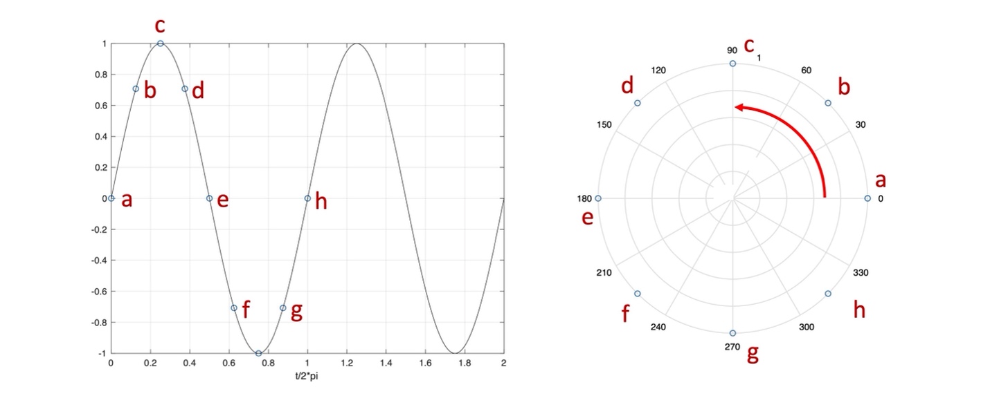
Figure 1: Two representations of a sinusoid.

The angular frequency reflects the same rate of change, but now expressed in radians per second.^[3] The 2 in Equation (1) equals the number of radians in one period of the waveform. Sometimes it’s more convenient to use one or the other. Irrespective of which one we use, they are both temporal frequencies – quantities that describe time-dependent behavior.

The relationship between wavelength and wavenumber k is

(2)

If we think of the wavelength as a spatial analog of the period T, then wavenumber is a spatial frequency.

With these definitions out of the way we can consider a familiar type of wave: sound in air. For sound waves, the relationship between angular frequency and wavenumber is given by

(3)

.

This equation has the form = f(k), which is called the dispersion relation for a particular wave medium – such as sound waves in air, surface water waves, flexural waves on a plate, etc. – and wave type. The dispersion relation specifies how the temporal and spatial frequencies inter-relate for a given system. For sound in air this relationship is rather simple, and linear to boot.

From the dispersion relation we can derive the phase speed of these waves – the speed at which any single frequency or pure tone component travels – by dividing both sides of Equation (3) by the wavenumber k, yielding

(4)

.

We can also derive the group velocity of sound waves – the speed at which a combination of tonal components travels – by differentiating Equation (3) with respect to k, yielding

(5)

.

Equations (4) and (5) tell us some important things about sound waves. First, the phase and group velocities are equal. This means a complex sound, such as the combination of tones from a band comprised of various musicians playing different instruments, will have all its components arrive at the listener at the same time; what is sometimes called in phase. We’ll call this collection of tones a group.

Imagine a band playing a song, where a bass guitar note, a guitar note, a snare drum hit, and a cymbal strike all occur at the same time. What it would be like if the sound from each of these traveled at a different speed, rather than together as a group? Music would be an incoherent mess, and it would be messier the further the listener sat from the band as the various components move further out of phase with each other. Every tonal component of music travels at the same speed in air, and any group of tones does as well. They do not disperse (de-cohere) over time and distance and are thus called non-dispersive.

Equations (4) also tells us is that sound’s frequencies and wavelengths are inversely proportional to each other. For a given sound wave speed c, if the frequency increases the corresponding wavelength must decrease so that their product remains constant. Remember, a sound waveform comprised of several tonal components must move as a group no matter what its frequency / wavelength content. And since sound’s phase and group velocities are equal this relationship holds for individual tones / wavelengths as well as any combination.

With these preliminary concepts out of the way, we can return to our favorite medium for wave propagation: the water’s surface.

Water Waves

In this section we’ll compare low amplitude surface waves on shallow water, and on deep water. “Low amplitude” means that the wave height is small compared to any surface wavelength. This yields a simpler, linear model; we’ll save the nonlinear model for the next section. “Shallow” means that the water depth D is less than half a wavelength, which we derived in Part 4. We’ll see that linear shallow water waves behave in many waves like sound waves in air.

The dispersion relation for low-amplitude waves on shallow water is given by

(6)

,

where g is the gravity constant. Using our tools from the previous section, the phase speed, e.g., the speed of any individual sinusoidal wave component, is Equation (6) divided by k,

(7)

.

This means that the phase speed is independent of wavelength on shallow water. The group velocity is found by differentiating Equation (6) with respect to k,

(8)

.

We see, then, that shallow water waves are not dispersive since neither wave speed depends on wavenumber (or, if your prefer, it does not depend on wavelength). Their wave speed only depends on the gravitational constant and the water’s depth. The various wavelength components of a wave group will travel together, and the composite wave shape doesn’t distort. An exemplary wave group is illustrated by the waveform plotted in Fig. 2; you can just as easily construct others as long as they satisfy the assumptions of the analysis. In this figure the solid black line is the wave group’s shape, while its components are the four other sinusoids.^[4] This shape would move unchanged in shallow water.

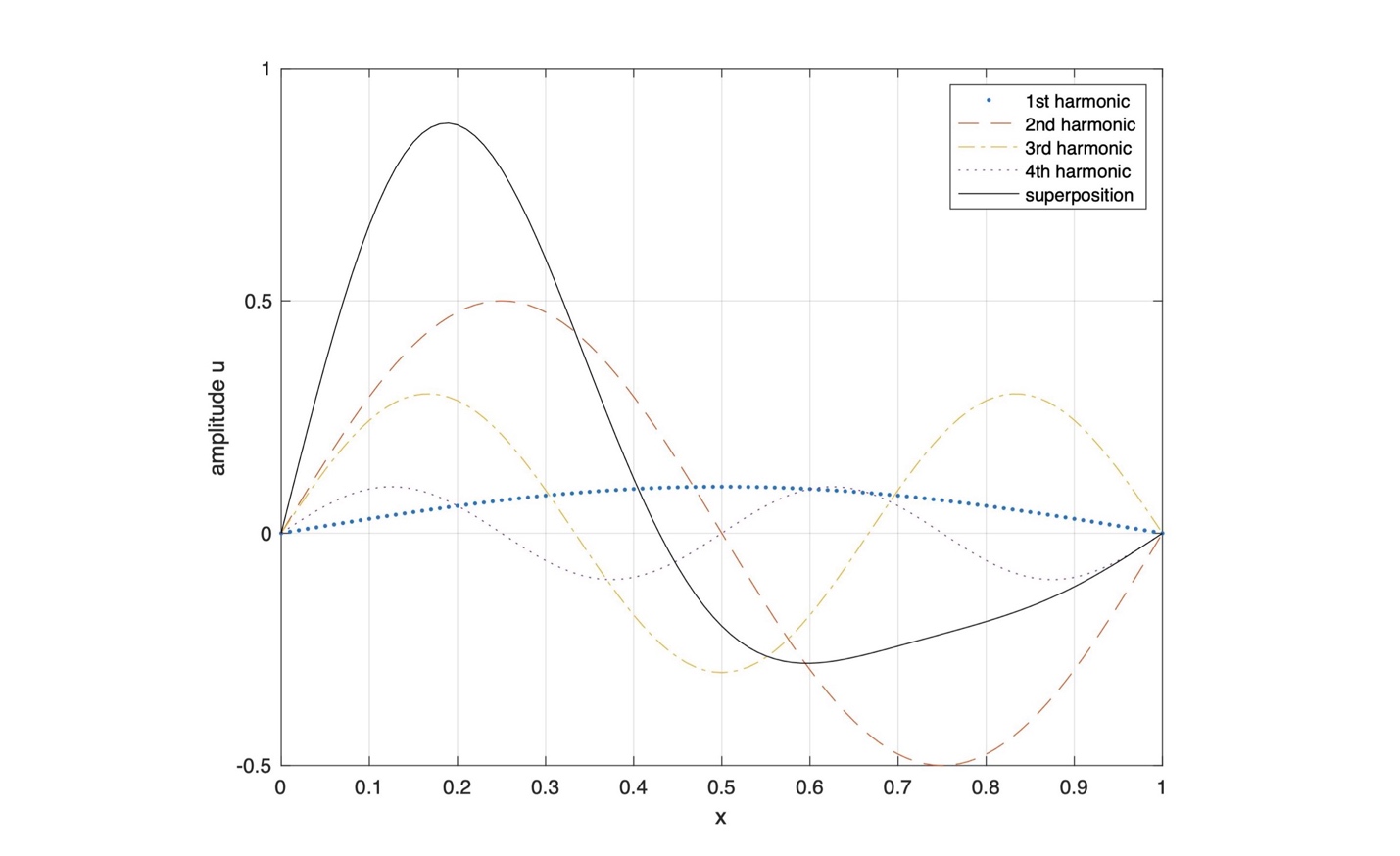
Figure 2: Wave group superposition and its components.

This wave group shape u in this Figure is the superposition of four harmonic component waves, expressed by

(9)

The wave’s components are computed at some arbitrary time t = 0; any time value will suffice since the wave components and their superposition merely translate along the water’s surface at the phase velocity (which here equals the group velocity).

Things are different in deep water, e.g., where the depth D is much greater than the wavelength. The dispersion relation for low-amplitude waves on deep water is

(10)

,

where g is the gravity constant and k is the wavenumber. The phase speed c_p for these deep-water waves derived by dividing Equation (10) by k,

(11)

,

While the group velocity is found by differentiating Equation (10) by k,

(12)

.

Comparing Equations (11) and (12) shows that the group velocity for linear deep-water waves is half the phase velocity. Also, the phase and group velocity of each wave component vary as the square root of the wavelength, or inversely as the square root of wavenumber. This means that deep water wave propagation is dispersive. Longer waves travel faster, which you have likely observed sitting on a lakeshore watching a powerboat’s wave train approach; the long waves arrive first. And any wave group comprising components with different wavelength will distort (e.g., de-cohere) over time and distance. This decoherence is plotted in Fig. 3 for the wave group defined by Equation (9), viewed from a fixed spatial position. Moving from the front curve toward the back, e.g., with increasing time, we see that the “sharper,” shorter wavelength components are being left behind by the faster long-wavelength components. Deep water waves are dispersive; shallow water waves are not.

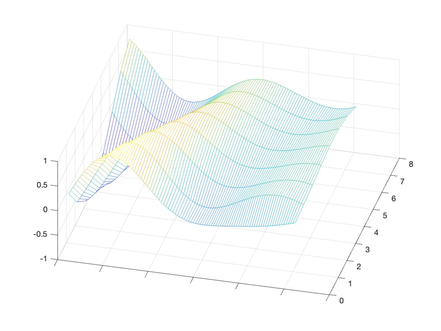
Figure 3: Wave group in deep water over time.

But what about shallow water nonlinear waves, where we don’t make the same small-amplitude assumptions required for linear surface wave theory? To answer that question, we’ll have to go back in time. Back to 1834, and to a canal near Edinburgh, where a young Scottish engineer was trying to determine how to make towed canal boats more hydrodynamically efficient.

Nonlinear Solitary Waves

In 1834, while conducting experiments on the Union Canal at Hermiston, Scotland to determine the most efficient design for canal boats, an engineer named John Scott Russell made a remarkable discovery. I’ll let him describe it in his own words:

I was observing the motion of a boat which was rapidly drawn along a narrow channel by a pair of horses, when the boat suddenly stopped – not so the mass of water in the channel which it had put in motion; it accumulated round the prow of the vessel in a state of violent agitation, then suddenly leaving it behind, rolled forward with great velocity, assuming the form of a large solitary elevation, a rounded, smooth and well-defined heap of water, which continued its course along the channel apparently without change of form or diminution of speed. I followed it on horseback, and overtook it still rolling on at a rate of some eight or nine miles an hour, preserving its original figure some thirty feet long and a foot to a foot and a half in height. Its height gradually diminished, and after a chase of one or two miles I lost it in the windings of the channel. Such, in the month of August 1834, was my first chance interview with that singular and beautiful phenomenon which I have called the Wave of Translation.^[5]

Russell’s Wave of Translation is a coherent wave phenomenon displaying many properties of a particle. In modern parlance we call his wave a soliton, a self-sustaining wave packet of constant shape that propagates with a constant velocity. In addition to surface water waves, solitons represent the behavior of nonlinear optical systems used in telecommunications, plasma dynamics, shock waves, and planetary gas dynamics (including Jupiter’s Great Red Spot).

Russel plotted the wave shapes he observed on the canal, and carefully documented their characteristics. The series of plots shown in Fig. 4 shows some of what he saw.

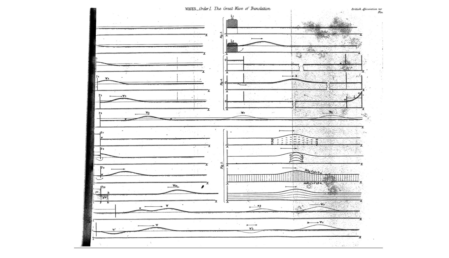
Figure 4: Excerpt from Russel’s study of canal waves.

These wave shapes may remind open-water paddlers of near-shore wave trains in shallow(er) water, as shown in Fig. 5.

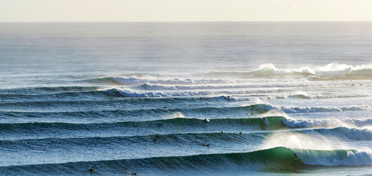
Figure 5: Wave train approaching shore.

Russel also documented ocean waves like these, noting that they broke at inflection points of the bottom bathymetry, and then established a regular periodicity and unique shape without dispersion as they continued toward shore:

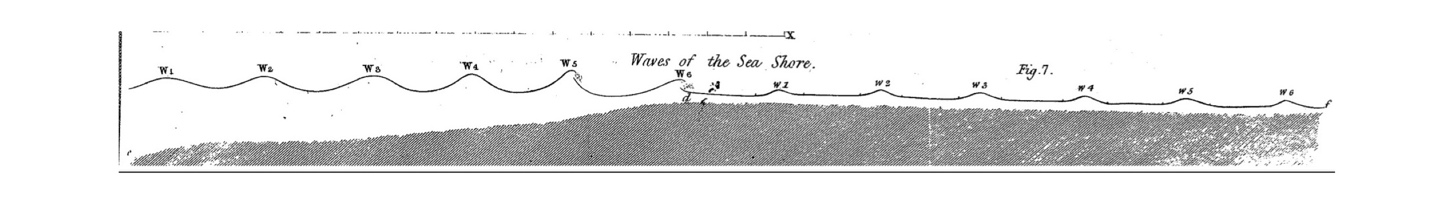
Figure 6: Russel’s cross-section of ocean waves approaching shore.

Those of us who’ve paddled in the shallows of freshwater rivers will also recognize these types of steepening waves. Depending on the water depth they may travel faster than we typically can paddle. If we “pop” our hulls and get on top of them, we can drop nearby boats in a flash.

The shallow water wave shapes depicted in Figs. 4, 5, and 6 all have the following characteristics: symmetry back-to-front, no dispersion since they maintain their shapes, and a waveform shape that drops on either side of its peak amplitude. Russell also noted that these waves have a speed that depends upon the water’s depth, as well as the wave’s amplitude, with taller waves moving faster than shorter waves. Linear waves do not display this type of amplitude dependence.

Many of Russell’s contemporaries doubted his results. These included Sir George Airy, a member of the Royal Society and England’s Astronomer Royal after whom the Airy equation and Airy functions are named, and Sir George Stokes, Lucasian Professor of Mathematics at Cambridge – the same chair first held by Isaac Newton, and later by Stephen Hawking – who along with Claude-Louis Navier developed the Navier-Stokes equations, which are the basis of contemporary fluid mechanics modeling and analysis. That’s some name-brand opposition! Their objections were primarily based upon mathematical analysis: they had not derived mathematical models of surface water waves that displayed this behavior. While I have deep respect for Airy’s and Stokes’ contributions and legacies, I think they should have gotten out of the office more. Russell, it turns out, was spot on in his observations. It just took a more sophisticated mathematical model to capture this real-world behavior.

J.W.S. Strutt (aka, Lord Rayleigh) and Joseph Boussinesq made further inroads into this problem, whereupon Diederik Korteweg and Gustav De Vries developed a mathematical model in 1895 for Russell’s Wave of Translation. The so-called Korteweg-De Vries (‘KDV’) equation is a nonlinear partial differential equation. While they were able to infer certain characteristics of the solution to this equation, it was not fully solved until the 1960s. The most well-known solution, which prescribes the shape of the waveform Russell observed, is represented by a function which varies over space x and time t given by

(13)

where the various constants are expressed in terms of the gravitational constant g and the water’s depth D by

(14)

.

An example of this waveform is plotted in Fig. 7. Note the correspondence to Russell’s plots in Figs. 4 and 6.

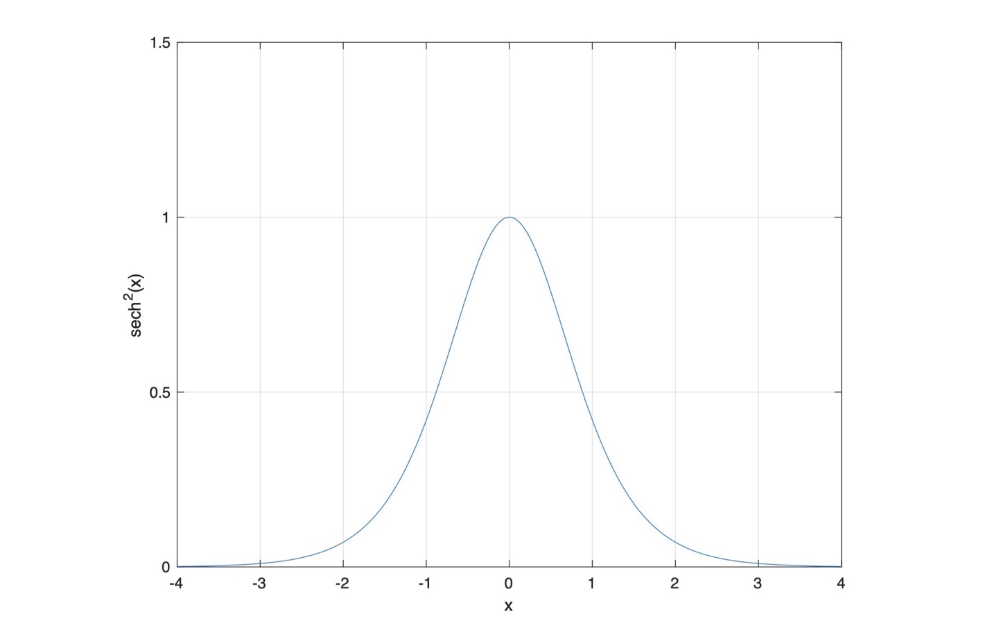
Figure 7: Plot of a hyperbolic secant function squared.

This wave moves at a speed U defined by^[6]

(15)

,

where A is the wave’s amplitude. This shows that the wave speed depends upon the wave’s amplitude, with taller waves moving faster. Amplitude dependencies and couplings like this are found in many nonlinear systems. Further, note that the wave is non-dispersive since its wave speed does not depend on wavelength / wavenumber.  It is a nonlinear solitary wave, or soliton.

While the KDV equation models behavior that paddlers experience, it does not model wave breaking. In essence, the KDV equation incorporates the next level of complexity compared to linear surface wave theory, but only the next level. Breaking waves do not embody the limitations and simplifications invoked even in deriving the KDV equation.

Summary

In this installment of the Science of Paddling series we haven’t done any paddling.  We’ll save that for the next article.  Instead, we reviewed several concepts from the science of wave propagation. Some of the topics are just fun, like why a circular frequency is called circular.^[7] Others give us context for what we observe in nature, such as why the long wavelength portion of a powerboat wake arrives first across a deep like. Plus, it’s enjoyable to see a perspective into 19^th century science, where so many things we now take for granted were initially wrestled with.

Science is really two complementary processes: analysis and synthesis. Based upon observations in the physical world we try to decompose things into their component parts, which (hopefully) are parts we understand. That’s the reductionist part I alluded to in the Introduction. Then we work to understand how those parts function together to produce the stuff we observe. That’s where the KDV equation comes from, for example. It’s a model expressed in the language of mathematics. Working with these models we can more deeply understand properties of the system that we have seen, such as wave dispersion and solitary wave formation. That’s the ‘why’ part, and the through line for all TSOP articles: the why. And if we’re both insightful and lucky we may understand the system enough that we can produce results that we haven’t experienced before, such as working with surface waves to do fun stuff like surf, or design a more efficient hull. That moves us from science to satisfaction, perhaps even to fun. Who wouldn’t want that?

Extra Credit: The Korteweg-De Vries Equation

The Korteweg-De Vries (‘KDV’) equation, which represents one-dimensional shallow water surface waves, is given by

(16)

,

where , , and are constants defined by

(17)

.

In these equations u is the wave’s height about a nominally flat-water surface, x and t are position and time, g is the gravitational constant, and D is the water depth.

Equation (16) is a partial differential equation; the second term’s product of u and its spatial derivative makes it nonlinear. Fortunately, we can infer the form of the solution based on the physical properties of Russell’s Wave of Translation. We know from experience that these waves have a localized peak height, and that this height decreases away from the peak both behind and ahead of the wave. Mathematically we would state that the value of u an infinite distance from the peak wave height goes to zero, along with its derivatives. This lets us prove that the solution to the KDV equation is uniquely determined by initial conditions.^[8] We also know that the wave maintains its shape, e.g., it is not dispersive.

Since Russell observed the Wave of Translation propagated along the canal’s surface, we can conclude that the solution to the KDV equation takes the form

(18)

,

where f is some function, to be determined, that describes the wave’s shape. Equation (18) is a so-called d’Alembert or traveling wave solution. Because the wave is non-dispersive the shape of the wave f must be the same for all values of space x and time t. Certainly, if the argument of the function, (x – Ut), does not change as the wave travels in space and time, f won’t change either. One way to keep the argument from changing is to pick the parameter U so that

(19)

.

We see then that U is the wave’s speed, the proportionality constant relating distance traveled and time. As the wave moves over increasing distance x, time t must increase proportional to the speed U to maintain a constant argument and thus preserve the wave’s shape. This means the wave described by Equation (18) is moving left-to-right in our coordinate system.^[9]

The solution to the KDV equation is given by

(20)

for

(21)

.

A is the wave’s height, which is determined by initial conditions. The function sech is the hyperbolic secant function. No need to panic; the hyperbolic secant is just a convenient way to express a combination of exponentials:

(22)

.

If we combine Equations (17) and (21) we have an expression for the wave speed U in terms of the gravity constant and depth,

(23)

.

This means the soliton’s speed depends on the water depth D as well as the wave’s amplitude A. The greater the amplitude, the faster the wave propagates.  By contrast, linear waves do not have amplitude-dependent speeds.

We can re-write Equation (23) as

(24)

.

When the wave amplitude A becomes much smaller than the depth D this reduces to the shallow water linear wave speed we studied in Part 4,

(25)

.

Equation (25) in light of Equation (24) reinforces how the linear wave approximation we considered in Part 4 is indeed a small-amplitude solution.

REFERENCES

James Lighthill, Waves in Fluids, Cambridge University Press, 1^st Edition (1978).

J. Scott Russell, “Report on Waves,” Report of the Fourteenth Meeting of the British Association for the Advancement of Science, pp. 311-390 (Sept. 1844).

George Carrier and Carl Pearson, Partial Differential Equations: Theory and Technique, Academic Press, New York (1976).

G.B. Whitham, Linear and Nonlinear Waves, John Wiley & Sons, New York (1974).

© 2022, Shawn Burke, all rights reserved. See Terms of Use for more information.

1. “OK, stuff is made of molecules. But what are molecules made of? OK, molecules are made of atoms. But what are atoms made of? OK, atoms are made of quarks and leptons. But what are quarks and leptons made of?” ↑
2. Bonus points to anyone out there who has gone to the Muddy Charles pub. ↑
3. You may recall from high school geometry or trigonometry that 360 degrees of arc equals two pi radians. ↑
4. Those of us in the biz refer to this type of representation, or decomposition into distinct waveform components, as a Fourier series. ↑
5. J. Scott Russell, “Report on Waves,” Report of the Fourteenth Meeting of the British Association for the Advancement of Science, pp. 311-390 (Sept. 1844). ↑
6. Note that a soliton has one wave speed since the soliton wave moves as one entity. You might infer this means its group and phase speed are equal, but tread carefully there. That question opens up an entire branch of wave propagation theory involving cnoidal waves and other fun stuff. ↑
7. Or at least I think it’s fun. Your mileage may vary. ↑
8. This is not true for many nonlinear systems. For some interesting examples see James Gleick’s book Chaos. The uniqueness proof is well beyond the scope of The Science of Paddling. ↑
9. If instead the argument were (x + ct) then the wave would be moving right-to-left; the proof is left as an exercise to the reader. ↑