By Shawn Burke, Ph.D.
OVERVIEW
Hooke’s Law is reviewed as an approach to indirectly estimate paddling force. A simple, qualitative technique for making this measurement in the field is presented. The technique is suitable for kids and families; you can be a scientist.
THE FORCE IS WITH YOU… AND AGAINST YOU
Last year a noted surfski paddler emailed and asked if Newton’s 2nd Law could be used to estimate paddling force, i.e., the integrated force applied by a paddler through the blade into the water. Naturally I ran with the idea since it offered the possibility of inferring paddle force using only an accelerometer. However, physics hit me right between the eyes. As you may recall from Part 14: Kind of a Drag, there are actually three forces at play when moving a hull: paddling force F, total mass m and acceleration (e.g., the time rate of change of velocity v), and the drag force:

If the coefficient of drag Cd were zero (1) Newton’s 2nd Law would directly apply, and (2) it would only take one stroke to complete a race since, in the absence of drag, you’d never slow down. If we were only so lucky!
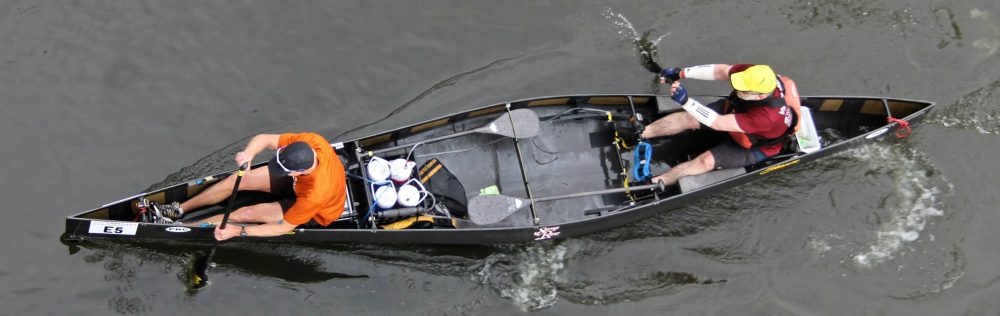
So instead, is there a situation where the inertial term is zero, or nearly so? And where the drag force is zero, or nearly so? Well, sure; as long as you’re not moving. And the best way not move when paddling is to be tied to an anchor. This may sound silly, but it’s not. Because if you can measure the force transmitted into the anchor from the paddled hull, you have a way to indirectly infer the paddling force. This is because Newton’s First Law teaches us that if a force is being applied, but you’re not moving, there must be an equal and opposite force resisting your applied force.
To measure this force you could invest in a load cell, a strain-gauge-based device that provides a signal output proportional to the force applied through[1] it. You might have a spring-based weight scale. Or, you could take advantage of Hooke’s Law and do it on the cheap, as we’ll see.
GETTING HOOKED
Back in 1676 English physicist Robert Hooke noted the relationship between the deformation (e.g., stretching) of a spring and the load applied to it. Since it was the 17th century, he did so in Latin: “Ut tensio, sic vis” (“as the extension, so the force”)[2]. This means, quite simply, that the extension of a spring ∆ is linearly proportional to the applied force F:

The proportionality factor k is called the “spring constant.” The force can be a weight hanging from a fixed spring, as shown in Fig. 1. One sees that by knowing the spring constant (or determining it by calibration), and measuring the deflection ∆, one can then infer the applied force using the equation above.
![]()
Figure 1: Weight W elongating a spring by the amount ∆.
There are some assumptions inherent in this linear model. First and foremost is the assumption that the spring is linear! In the real world no spring is truly linear. When enough load is applied to a spring it will either break (which is represented mathematically by the spring constant abruptly going to zero, an extreme example of a so-called “softening” spring), or it will stiffen up and no longer deform as the applied load is increased (e.g., it becomes nonlinear, in this case a “hardening” spring) – then it will break as the load is increased. But as long as you operate in this linear range you can rely on this simple model to predict how a spring will deflect subject to an applied load. Or, given how much a spring stretches when subject to an applied load, and the spring constant, what that applied load is.
LET’S GET ON THE WATER
So, got any springs lying around the house? Ever heard of a bungee cord?
Imagine tying one end of a bungee cord – or a set of bungee cords connected in parallel[3] – to the stern of a canoe, kayak, surfski, or SUP. And tying the other end to a fixed anchor like a dock or a tree, as suggested in Fig. 3(a). If the bungee cord is too short to span the distance between hull and anchor a non-stretchy rope may be used to extend it. Also – and this is very important – the bungee cord(s) must be chosen such that they are stretched in their linear range in step (c) below, which argues for a set of bungees in parallel. (You’ll have to experiment a bit since the stretchiness of bungee cords is highly variable.) This is because the equivalent stiffness of bungee cords in parallel is equal to the sum of their spring constants,

e.g., the stiffness of the set is greater than the stiffness of its component elements; the equivalent stiffness of springs in series is actually less than the stiffness of its component elements. An example of bungee cords assembled in parallel is shown in Fig. 2. The ends were gathered using a wire tie; you’ll probably need more than two in a bundle!
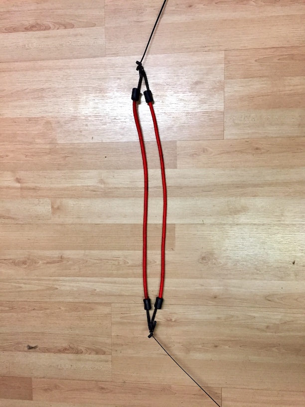
Figure 2: Bungee cords in parallel.
Next, the paddler gently eases the hull away from the anchor so as to take out any slack, as shown in Fig. 3(b). At this point, an assistant on shore measures the length of the bungee cord (or cord + stiff rope). This establishes the baseline length D. This measurement can be made by connecting a sufficient long tape measure to the stern and letting it pay out; you could even use a string. Or, the “no slack but no load” location can be marked with tape on a dock adjacent to the hull.
Then the fun begins. Note before you start that the hull is likely to bounce some front-to-back, especially for a single-blade paddler. (It feels a bit strange. Maybe more than a bit.) The paddler then… paddles, as suggested in Fig. 3(c). It’s best to ease into it with easier strokes before gradually performing progressively stronger strokes. The shore-based assistant notes the distance ∆ that the bungee cord(s) stretch. This is not an exact science; a little patience and willingness to experiment is required. But with a little practice you can get a qualitative measurement of “peak stretch” for a given paddler, hull, and paddle. And get a few laughs in the process. You may find the hull “bouncing” on the bungee. The best way to avoid this is with a stiffer bungee – or stiffer parallel set of bungees – for reasons illustrated in the Appendix.
Record the data, then the paddler and shoreline assistant switch roles and the process is repeated. The possibilities for bragging rights are endless.
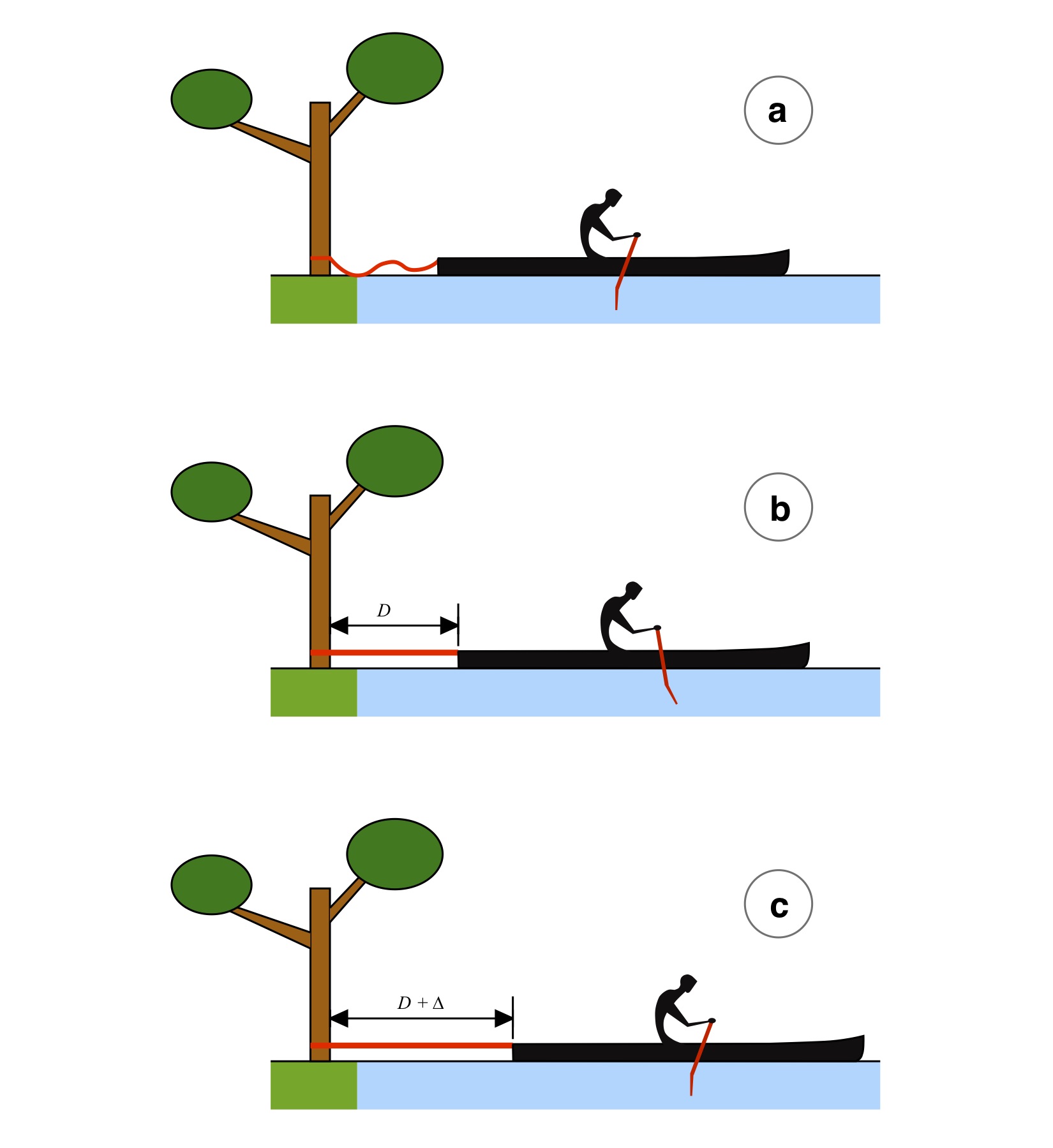
Figure 3: Paddler anchored to tree (a) with slack bungee; (b) without slack in bungee, but not yet stretched; (c) with bungee under load from paddling force.
BACK ON LAND
Now that you have your deflection data ∆, it’s time to calibrate your bungee cord(s). Take the same cord(s) you used in your field tests and fix one end to a ceiling rafter, strong tree branch, football goal posts, or whatever other strong and fixed anchor you can find. Let the cord(s) hang free, and note either their length, or their height off the floor / ground as suggested in Fig. 4(a). Then attach a known weight to the lower end and measure the deflection, as suggested in Fig. 4(b), with a real-world sample shown in Fig. 5.
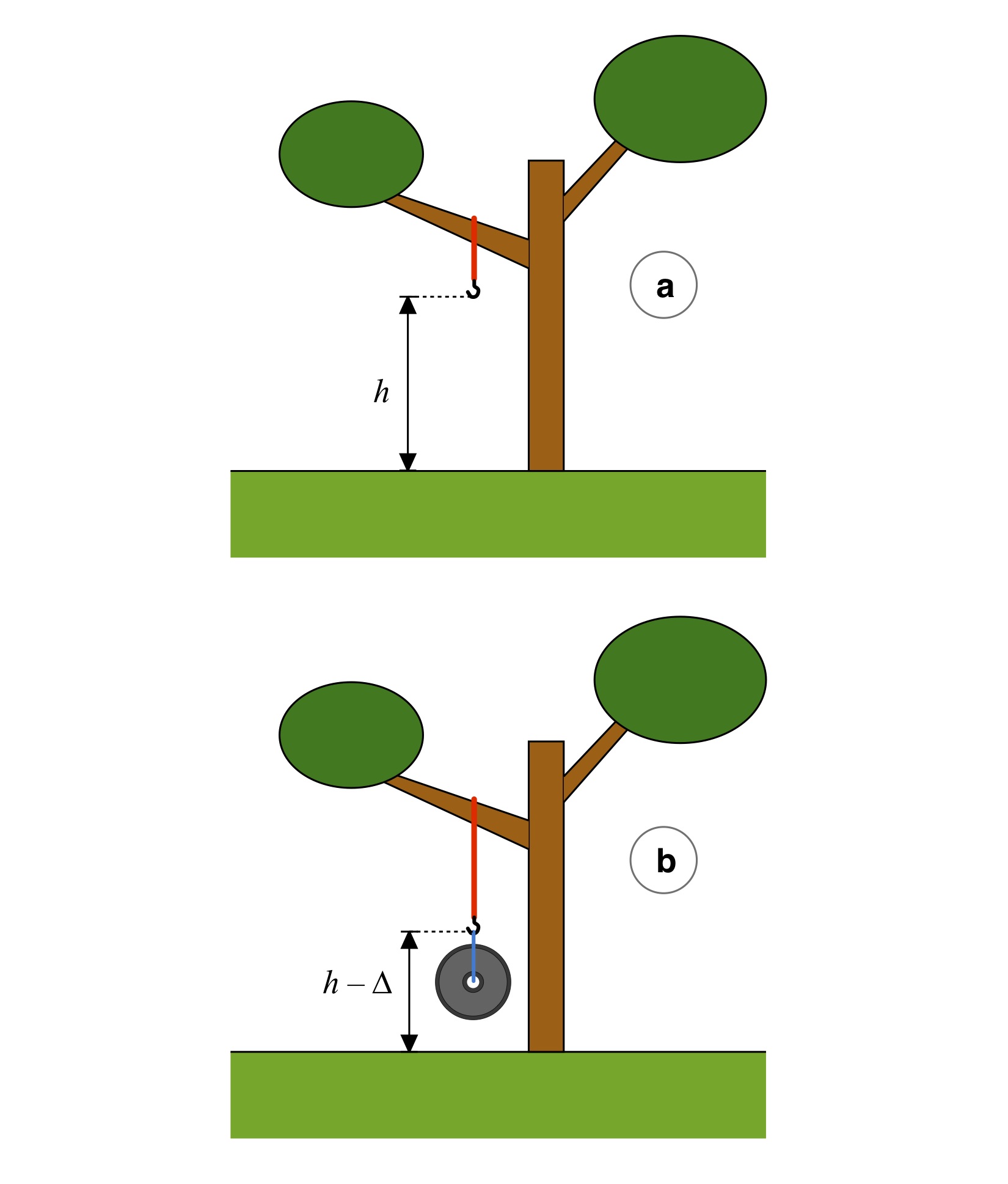
Figure 4: Calibration procedure: (a) unloaded baseline measurement; (b) loaded deflection measurement.
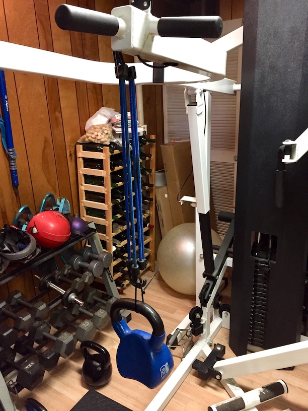
Figure 5: Calibrating a parallel group of bungee cords using a known weight.
If the world were perfect you’d only have to make this measurement with one weight since, in that perfect world, the bungee cord(s) would act like a linear spring, and your measurement would be made with unmatched accuracy and precision. So just in case, try making the measurement with a few different weights loading the cord(s). For each case, given the known weight (e.g., force) and deflection, use Hooke’s Law to calculate the spring constant k:

Average the results and use the average spring constant to infer the paddling force from Hooke’s Law
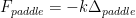
Then let the bragging begin!
SUMMARY
In this installation of the Science of Paddling series we’ve reviewed Hooke’s Law, and used it to develop an approach for indirectly estimating paddling force. A simple technique for making this measurement in the field was outlined. The technique is suitable for kids and families, which given how we’re all socially distancing may be a fun thing to try. Plus it gives us all a chance to be scientists, and learn a little physics along the way.
Just approach this with a sense of adventure, and a willingness to experiment. There is no one way to make this measurement. Also, keep in mind that paddling in a fixed frame – anchored in place – will both churn up water and alter your stroke mechanics. This makes it difficult to rigorously map paddle force results from this test to paddle force when the hull is free to move. But if done comparatively across a group of paddlers it provides an amusing way to compare “paddling strength.” Or perhaps who has the best technique for this particular configuration.h
Just be mindful of the bounce; choose your springs wisely (see the Appendix for how and why). And no cheating!
APPENDIX: THE SIMPLE OSCILLATOR
A canoe, kayak, surfski, or SUP attached to a fixed anchor via an elastic cord is a classic example of a spring-mass-damper system, otherwise known as a “simple oscillator” like that depicted in Fig. 5. A mass (the hull, paddler, and paddle) is attached to a fixed anchor via a spring. A linear damper with damping coefficient b is included as a simple model for energy loss in the system. The mass is free to move (a bit) in the horizontal (‘x’) direction.
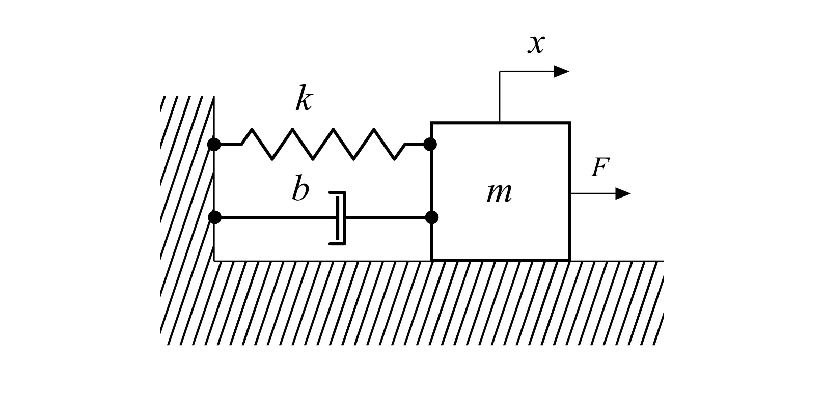
Fig. 5: Spring-mass-damper simple oscillator.
An exogeneous force F (the force exerted by the paddler through the paddle) acts on the mass. Using Newton’s First and Second laws, the governing equation for this system is

Dividing by the mass, this can be rewritten as
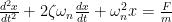
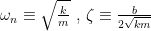
Where the angular natural frequency 
For continuous paddling, the paddling force can be represented as a combination of sinusoidal functions using Fourier superposition. For the sake of simplicity we’ll limit ourselves to the first term in this expansion, and represent the paddling force as a single sine wave input at angular frequency w with amplitude F0 via
Since the system is linear, and the input force is a sinusoid, the position of the mass over time x(t) must also be a sinusoid at the same frequency. The response will have an amplitude X, and phase shift 

Solving for the response amplitude in terms of the input force amplitude, and rearranging terms, yields a nondimensional way to express the hull’s response amplitude and phase to the paddling input. This response is called the frequency response function since it depends on the angular input (paddling) frequency 
![\frac{Xk}{{{F}_{0}}}=\frac{1}{\sqrt{{{\left[ 1-{{\left( \frac{\omega }{{{\omega }_{n}}} \right)}^{2}} \right]}^{2}}+{{\left[ 2\zeta \left( \frac{\omega }{{{\omega }_{n}}} \right) \right]}^{2}}}}](https://s0.wp.com/latex.php?latex=%5Cfrac%7BXk%7D%7B%7B%7BF%7D_%7B0%7D%7D%7D%3D%5Cfrac%7B1%7D%7B%5Csqrt%7B%7B%7B%5Cleft%5B+1-%7B%7B%5Cleft%28+%5Cfrac%7B%5Comega+%7D%7B%7B%7B%5Comega+%7D_%7Bn%7D%7D%7D+%5Cright%29%7D%5E%7B2%7D%7D+%5Cright%5D%7D%5E%7B2%7D%7D%2B%7B%7B%5Cleft%5B+2%5Czeta+%5Cleft%28+%5Cfrac%7B%5Comega+%7D%7B%7B%7B%5Comega+%7D_%7Bn%7D%7D%7D+%5Cright%29+%5Cright%5D%7D%5E%7B2%7D%7D%7D%7D&bg=ffffff&fg=000&s=0&c=20201002)
This function is plotted for a range of angular frequencies normalized by the undamped resonance frequency
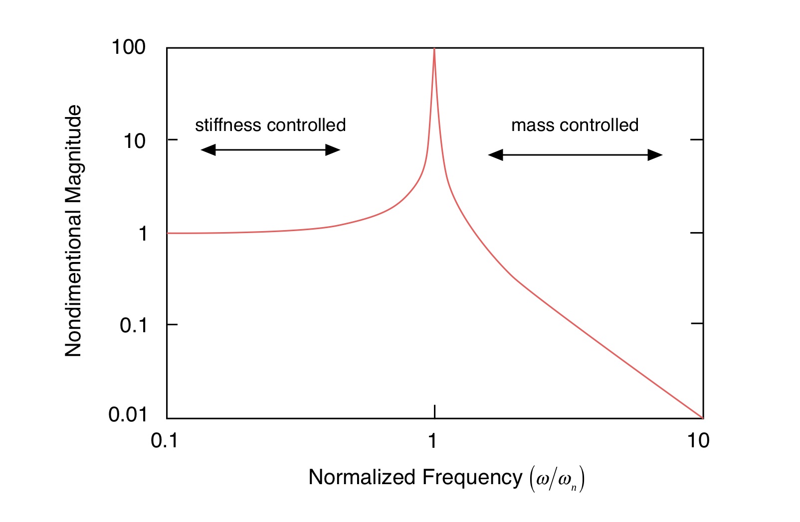
Figure 6: Magnitude response of a simple oscillator.
Most people have a stroke rate between 30 and 90 strokes/minute. In order to avoid any “bounce” when making the measurement described herein it’s best to move the resonance outside of the frequency range. In other words, move the resonance to the right. How do you do this? Recall that the undamped resonance is defined in terms of the square root of the ration of the spring constant divided by the mass. Since the mass of the hull/paddler/paddle is fixed, this means making the spring stiffer. Which means adding bungee cords in parallel to stiffen the elastic attachment to the fixed anchor. A load cell would have “infinite” stiffness (at least compared to a bungee cord), but who has one of those?
V1.0
© 2020, Shawn Burke. All rights reserved. See Terms of Use for more info.
- I use “through” rather than “to” so as to reflect the concept from linear systems theory that force is a “through” variable (analogous to electrical current)h, while velocity is an “across” variable (analogous to voltage). ↑
- Henry Petroski, Invention by Design: How Engineers Get from Thought to Thing, Harvard University Press. p. 11 (1996) ↑
- Bungee cords in series means bungees tied end-to-end. Bungee cords in parallel means laying them side-by-side, with the connectors gathered together at each end. ↑