Uncategorized | The Science of Paddling

by Shawn Burke, Ph.D.

SUMMARY

A handbook for reading the math in Science of Paddling articles. Not a primer on how to do math.

NOW ABOUT ALL THOSE EQUATIONS…

In a November 2019 poll of Science of Paddling readers 31.3% of you reported that the level of mathematical exposition in TSOP articles was just right. This means that 68.7% of readers are less than thrilled with the level of math presented:

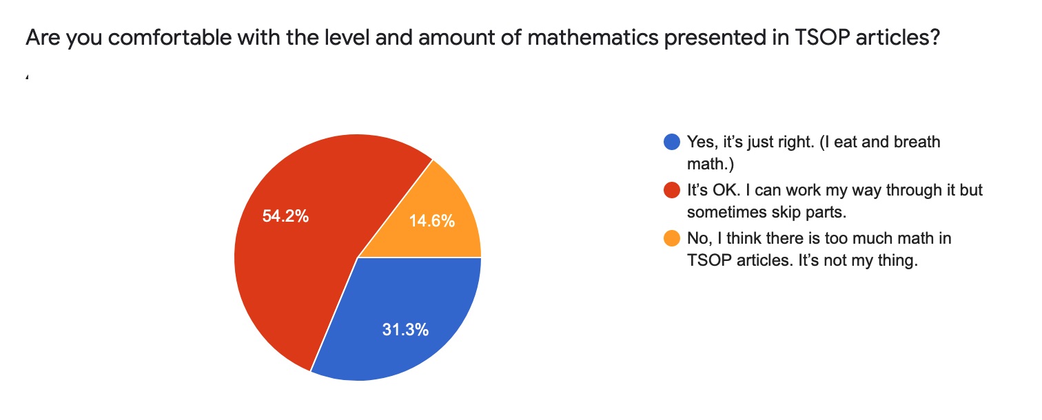
Figure 1: Survey results and question/answer wording.

As the late physicist Stephen Hawking noted in reference to his book A Brief History of Time, “Someone told me that each equation I included in the book would halve the sales.” Yet his book sold an astounding 25 million copies from 1988 through 2007. I’m not Stephen Hawking. But it appears that there is enough value in The Science of Paddling articles for readers around the world to willingly wade through the details in search of useful nuggets. Or perhaps just for the pleasure of learning new things.

Still, the one negative comment I periodically get about the article series is its reliance on mathematics; on “all that math.” That’s hard to avoid since the bulk of TSOP articles are grounded in physics and applied mechanics, and their language is… mathematics. I’ve found numerous write-ups in books, magazine articles, and on the web that describe the physics of paddling at a very high level, without any math. However, these expositions won’t get you much beyond “paddle force leads to a reaction force that propels the kayak,” and maybe a few arrows superimposed on a photograph of a paddled hull. I want to know more – to get at the why, and to explore more in-depth topics – and I believe readers want to know more as well. I could be all hand-wavy, drop the rigor, and ask you to just believe what I write. But I respect the subject matter more than that, and I respect you as discerning readers more than that as well. So I’m left with the convenient shorthand of science to clearly show the basis for why: mathematics.

But “all that math” needn’t be a mystery, a series of strange symbols and curlicues whose intent is to confound. Just think of mathematics as another language; a language you might not be very familiar with. Like all language math has rules, as well as dialects and idioms that spring from its varied sub-fields of practice and application. Learning just enough of its grammar, words, and phrases will help you navigate the landscape, facilitating a more immersive experience as you work your way through technical articles and books.

As an example, consider the language of equations. An equation expresses a concept; no mystery, that’s all there is to it. And they often do not lend themselves to linear thinking like, say, a computer program. An equation is more like someone describing an experience and the conclusions drawn from it, albeit in a rather precise and detailed way. For example, the equation

$F=\frac{1}{2}\rho A{{C}_{D0}}\cos \left( \theta -\phi \right)\left( {{v}_{hull}}-{{v}_{paddle}} \right)^{2}$

is another way of saying, “I pushed off with my paddle and the hull sped up.” It synopsizes the co-dependent relationship between paddle force F and the hull and paddle velocities v_hull and v_paddle. The rest is detail, such as the definitions of the constants and variables which are (or should be!) provided by the author, as well as some skill in looking at limiting cases; more on that below.

In order to understand what is being expressed in any equation there are a few rules that will help you read and understand its “words” and “grammar” in order to discern the insights expressed there. That’s the purpose of this installment of the Science of Paddling series. Think of this as a handy phrasebook for navigating articles in series.

To realize this we’ll hew to an adage from my 9^th grade Algebra II teacher, Mrs. Verna Hazen. Mrs. Hazen’s advice kept me and my classmates from getting bogged down in the “what is this?” of mathematics; like my 9^th grade self, we’re more interested in what math does. I’ll never forget her standing in front of the classroom, moving away from the windows toward the blackboard’s right side, pausing to consider her chalk-covered fingers, then looking up and saying, “Algebra is a game. And like all games, it has rules. If you follow these rules you will not have any difficulty with algebra.”

So let’s meet this challenge head on, and review the rules – the words, grammar, and syntax – used in the mathematics of Science of Paddling articles, along with examples. The goal isn’t to have you do math – leave that to me – but to read and get more from it. This isn’t a primer on how to read all mathematics; that would be unwieldy, overly broad, and beyond my expertise; we’ll be mindful to keep in our own lane.

What follows are a number of topics, covering variables, vectors, plots, functions, equations, and more, along with examples from the articles. There are a few sidebars that you can skip, or read if you’d welcome a bit more depth and historical context. While the topics are arranged in a more or less progressive order (since most math is built upon prior math), you can read them in order, or access any particular topic by clicking in the list below. Just remember that the art of reading mathematics requires some preliminaries. Your patience will be rewarded.

I look forward to speaking math with you soon.

TOPICS

Constants
Variables
Parameters
Symbols
Multiplication
Vectors and Scalars
Fractions
Powers and Roots
Functions
Plots
Derivatives
Summations
Integrals
Equations

Constants

We deal with constants all the time without giving them a second thought.

For example, we use numbers to count things, and the meaning of numbers – e.g., their value – does not change. It would be disconcerting to discover that there are suddenly 37 minutes in an hour because 60 and 37 exchanged places in our numbering scheme. While the more philosophical among you might contend that ‘37’ and ‘60’ are symbols that represent numeric quantities, we also share a social pact that specific numeric symbols have specific and unchanging meanings. Hence, constants.

The same agreement holds for quantities of measure like the meter (with symbol ‘m’), the second (with symbol ‘s’), or the liter (with symbol ‘l’). While typically employed to express quantities they too implicitly represent constants. And one quick way to tell if something is a mathematical constant or variable (but not a function) is to look whether it is written in italics. It’s a sure giveaway if textual convention is followed. Vector constants and variables have their won particular notation which we’ll encounter below.

Geometry provides us with the constant representing the ratio of a circle’s circumference to its diameter, $\pi$ , with value 3.14159265358…. Jacob Bernoulli^[1] gave us the constant e that forms the base of the natural logarithms and the natural exponential function, with value 2.7182818… You’ll find these two sprinkled throughout the articles.

Other constants have their origin in repeatable physical measurements. These include the acceleration of gravity on the Earth’s surface, represented by the symbol g; the density of water, typically represented by the Greek symbol $\rho$ (pronounced “rho”); and the kinematic viscosity of water, $\nu$ (pronounced “nu”). Curiously, these constants actually depend upon specific circumstances: the gravitational constant changes as we move away from Earth’s gravity well (thanks, Einstein!); the density and viscosity of water depend upon temperature. The only place where it is appropriate to equate g with 32.2 feet per second per second is on the Earth’s surface; values of water’s constituent properties are usually quoted at 20 degrees Celsius (68 degrees Fahrenheit) and must be adjusted otherwise. Still, we’re all paddling on the surface of the Earth, and the temperature of a lake or river (or the ocean) doesn’t change very quicky, so it’s reasonable to refer to these as constants

Variables

The number ‘6’ as written or spoken is a concept. It is a convenient shorthand to describe something we see or think about, like the number of bottles in a six-pack or the number of letters in the English word ‘friend’. We associate ‘6’ with a specific quantity or value. But what if I wanted to describe the number of spice jars in my pantry over time, the volume of gasoline in my car’s tank while I drive, or the number of letters in each of the words in the English language, e.g., a range of numbers? In that case we would use a variable.

A variable is one level of abstraction higher than writing a number like ‘6’. We generally represent variables using a letter, such as x or t. Conventionally the symbols x, y, and z represent a spatial location or direction; since there are an infinite number of spatial locations it makes sense to represent location compactly with a variable rather than via a very, very (very) long table of constant location values. The same goes for time, which can take on a range of values. By convention time t is expressed in relation to some fixed starting time or event. For convenience this starting time is usually (but not always) set to 0. We may define some initiating event, like the turning on of an applied force or the beginning of a particular phase of movement, as the t = 0 reference, much like race timing is done.

While variables are, well, variable, they nonetheless take on particular values, such as the average speed of a river at a particular time and place, or the force of a cross-forward whitewater paddle stroke in the middle of the power phase.

Within the context of functions and equations variables are either independent or dependent; more on this later.

Parameters

Parameters are variables that are set to a particular value, as if they were a constant, whereupon an equation is solved or a simulation is run to determine the influence of the parameter’s value. For example, in Part 11: About the Bend the bend angle of a bentshaft was studied parametrically (hence, parameter) over a few set angles to determine how it affected the synchronization of blade face angle, paddle force, and velocity in reference to the hull.

In the context of functions and equations parameters are always independent variables; they don’t depend on any other variable. They don’t have special symbols, and on their face look like any other variable. Parameters versus variables may sound like a distinction without a difference; the difference is in how the variable is used. The distinction affords precising in our writing.

Symbols

One typical stumbling block to reading mathematics is understanding Greek symbols. The simplest way to move past this hurdle is to realize that the Greek alphabet is just an alphabet, like the letters used in the English language are part of a Latin alphabet. They’re just letters: don’t overthink it. The Greek language was also used during the Renaissance for publishing scientific papers much like Sanskrit served as the academic language of ancient India. There is some historical precedent for using Greek symbology in technical writing.

Here are a few common Greek letters used symbolically in Science of Paddling articles along with their meaning:

$\rho$ (“rho”) – water density, a constant.

$\nu$ (“nu”) – water’s kinematic viscosity, a constant.

$\pi$ (“pi”) – the ratio of a circle’s circumference to its diameter, a constant.

$\theta$ (“theta”) – commonly used as a variable to represent angles.

$\phi$ (“phi”) – commonly used to represent an angular offset, such as a paddle bend angle. Electrical engineers will often use it to represent a phase lead or lag.

$\omega$ (“omega”) – commonly used to represent the so-called “angular frequency,” which is two times $\pi$ times the frequency (aka the “circular frequency”). Angular frequency pops up because of geometry and trigonometry, which measure angle in radians rather than degrees. There are 360 degrees in a circle, which equals one cycle (e.g., one time around the circle), and two times $\pi$ radians in that same circle. If one goes around a circle once per second the circular frequency is 1 Hertz^[2] (‘Hz’) or one cycle per second, which is equivalent to subtending two times $\pi$ radians per second in angular frequency. It is often preferable to represent frequency using w since it leads to more compact mathematical expressions where one would otherwise have to write 2 $pi$ f.

$\delta$ (“delta”, lower case) – commonly used to express an infinitesimal change in some quantity.

$\Delta$ (“delta”, upper case) – also used to express a change in some quantity, though not necessarily an infinitesimal change.

∂ (“del”) – another way to express an infinitesimal change in a quantity. Often found hanging around partial differential equations.

$\mu$ (“mu”) – typically used as a prefix in units of measure, such micro-meters (‘ $\mu$ m’), in order to denote one millionth.

$\tau$ (“tau”) – commonly used as a time variable, or to represent a lead or lag time.

Another confounding do-dad in mathematical notation is the subscript. Subscripts are merely helpful labels that allow constants or variables that are related to each other to be more easily grouped and identified. For example, a drag coefficient is usually written as C_D, while the drag coefficient for a paddle blade when oriented perpendicular to the water’s surface (or to an incoming flow) is C_D₀, with the ‘0’ indicating an angle of 0 degrees to the flow direction (aka, normal to the flow). Subscripts are handy for noting that a quantity is an average value, for example expressing an average velocity as u_avg rather than using the more arcane overbar notation.

Subscripts can be used to denote sequences of variables. For example, a sequence of N variables S₁ S₂ S₃… S_N can be written as S_i for i = 1…N (e.g., the index ‘i’ ranges from 1 to N).

Symbols are used to represent common mathematical operations and relationships. These include many familiar as well as some unfamiliar examples:

+ : addition

– : subtraction; also used to denote negative numbers (numbers less than zero)

$\times$ : multiplication; also see multiplication below for variants

÷ : division; also see fractions below for variants

= : equal to

≈ : approximately equal to

≠ : not equal to

< : less than, e.g., the quantity on the left side of the ‘<’ symbol is less than the quantity on its right

≤ : less than or equal to

« : much less than

> : greater than, e.g., the quantity on the left side of the ‘>’ symbol is greater than the quantity on its right

≥ : greater than or equal to

» : much greater than

± : plus or minus, either denoting both positive and negative values of a quantity, or a range such as for an error band

→ : goes to, as in the quantity on the left goes to (or approaches) the quantity on the right. Often used in describing limits or limiting cases.

‘ : an apostrophe usually referred to as “prime.” Generally signifies to a variant version of some quantity or function but is also used in many applied math texts to denote differentiation with respect to an independent variable. We use the former here, not the latter.

∞ : infinity, the number which has no number larger than itself

(), [], {} : parentheses, brackets, and braces are used to enclose collections of operations, functions, constants, and variables. Sometimes this is done because of mathematical necessity when the items inside need to be evaluated separately from other things. They also enable convenient groupings of terms that have some significance, physical or otherwise, like the difference between two velocities. Formally I was taught that you used parentheses first, then if you needed some other “enclosure” to group things that included quantities in parentheses you used square brackets, and if you needed a groups of things already in both of these you used curly braces. These days many apps for formatting math equations just use larger and larger parentheses. Go figure.

More specialized symbols for operators, and their uses, are defined below.

Multiplication

Why can’t we settle on just one way of expressing multiplication? I have no idea. Sometimes multiplication is written in the familiar way, such as 2 $\times \pi$ to denote two times pi. Other times symbols are placed adjacent to each other to signify multiplication, such as 2 $\pi$ . And finally, a dot (‘•’) can also represent multiplication, via 2• $\pi$ . Wouldn’t it be nice to settle on just one way of writing this? Yes, it would. Sorry.

Vectors and Scalars

Any variable that requires reference to a direction in its definition, or more than one dimension, is a vector.^[3] Vectors have both magnitude and direction. Everything else is a scalar, which has magnitude but no direction. For example velocity is a vector with speed as its magnitude, although the two are sometimes conflated (oops!). Constants like the acceleration due to gravity and the density of water are common examples of scalars. And not to confuse things, but… when all variables represent quantities that move in only one direction the variables are often treated as scalars even though there is a directionality – this often leads to speed being conflated with velocity in 1D. This may all sound like “How many angels can dance on the head of a pin?” but for the sake of precision I had to cover it.

Many people think of vectors as “arrows,” in that an arrow has a length and points in a certain direction – a reasonable analogy. The length corresponds to the vector’s magnitude; magnitude is a scalar. The vector variable’s dimensions along each axis of the coordinate system in which it is defined are its components. This is illustrated in Fig. 2 for a force vector F; note that vector variables are generally written in boldface. In 2D the projection of the vector’s length on the x– and y-coordinate axes are its components F_x and F_y in these directions; in 3D projecting the vector’s length onto the z-coordinate axis yields F_z. Again, these are its components.

By convention, a fluid velocity vector V has components in the x, y, and z directions written as u, v, and w. So if you see those, now you know.

As an aside, the organization of the coordinate system for a vector in 3D is important if you want the components you derive from it to be accurate. Take your right hand, extend its fingers, and imagine that your wrist is at the origin of the 3D coordinate axes (where the coordinate axes intersect). Extend your thumb upward, and orient your hand so that your palm and fingers are aligned with the x-axis. Now rotate your hand about the wrist counter-clockwise 90 degrees. Your fingers now point along the y-axis, and your thumb points upward along z-axis in its positive direction. This is the so-called right hand rule. Why is this important? I had a Summer job where my project’s lead engineer had defined the coordinate system for a skyscraper under development with the z-axis pointing the wrong way. We were measuring structural and façade loads on models of the building in a wind tunnel, and if we hadn’t corrected this axis definition it might have affected the real building’s structural design. Math counts, folks.

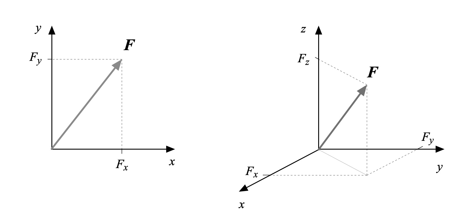
Figure 2: Vector F and its components in 2D and 3D.

Fractions

I first encountered fractions in grammar school; I expect most of you had a similar experience. Fractions are another way of representing division without actually performing the operation of dividing. Sometimes this is for convenience; other times, theater. But each of the following fractions serves a particular purpose:

$\frac{1}{4}$

$\frac{\rho}{2}$

$\frac{1}{x}$

In the first you can associate ¼ with dividing a whole (the “1”) into four parts. Simple. In the second the symbol $\rho$ , likely the density of water, is left “whole” in the numerator because in reading this fraction, plus any other mathematical terms that might adjoin it in a function or equation, the reader can keep in mind the physical association of mass per unit volume with the symbol $\rho$ . This provides more meaning than looking up the density of water in a table, dividing by two, and writing “0.49901 g/cm³ @ 20C “instead.

In the third fraction we have our initial introduction to really reading mathematics. One of the superpowers granted to those who take the time to actually read mathematics is the ability to explore the implications of what is written. Let’s assume ‘x’ is a variable in the third fraction’s denominator above. What are the consequences?

You might ask, “What do you mean by implications? It’s just a fraction!” Sure, it’s just a fraction. But what value(s) does the fraction take as the variable x changes? When x equals 1 the fraction equals 1 – check. When x becomes smaller than 1 the fraction becomes greater than 1 since dividing a number (here, the numerator) by a smaller number (here, the denominator) leads to a result that is greater than 1. As x becomes smaller and smaller the fraction becomes larger and larger; try a few values for x and see. As x approaches 0 the fraction becomes huge; in the limit it becomes infinite. If instead x becomes larger than 1 the fraction becomes less than 1 since dividing a number (here, the numerator) by a larger number leads to a result that is less than 1. As x becomes larger and larger the fraction becomes smaller and smaller; try a few values for x and see. And in the limit as x approaches infinity the fraction goes to zero. Finally, if x is a negative number then the fraction is negative as well.

This exercise is an example of reading mathematics. Rather than glossing over the fraction 1/x we spent a little time exploring its implications in light of the variable denominator. You can similarly investigate fractions with variable numerators, or where both numerator and denominator are variables. Mastering just this one skill of active reading will take you very far in extracting meaning from what might otherwise be a jumble of symbols and squiggles on the page. Don’t underestimate its power to inform.

Powers and Roots

One bit of notation you’ll see sprinkled through TSOP articles is a constant or variable with a numeric superscript, like x² or v³, or even L^2/3. These superscripts (generally) represent a power of the constant or variable; you’ll sometimes encounter the term “raised to the power of…” to signify this operation. Two common powers even have their own names: x² means the variable x is “squared,” or twice multiplied by itself; v³ means v is “cubed” or multiplied three times. The superscript number is termed the exponent. When the exponent is a whole number it represents the number of times the constant or variable is multiplied by itself.

Ever wonder where the terms “squared” and “cubed” came from? If you take a number and square it the result is a square with area equal to the result; if you were to cube it the result is a cube with volume equal to the result. These are illustrated in Fig. 3 for the square of 2 (area = 4, which you can prove for yourself by counting) and the cube of 3 (volume = 27, which you can also prove for yourself by counting).

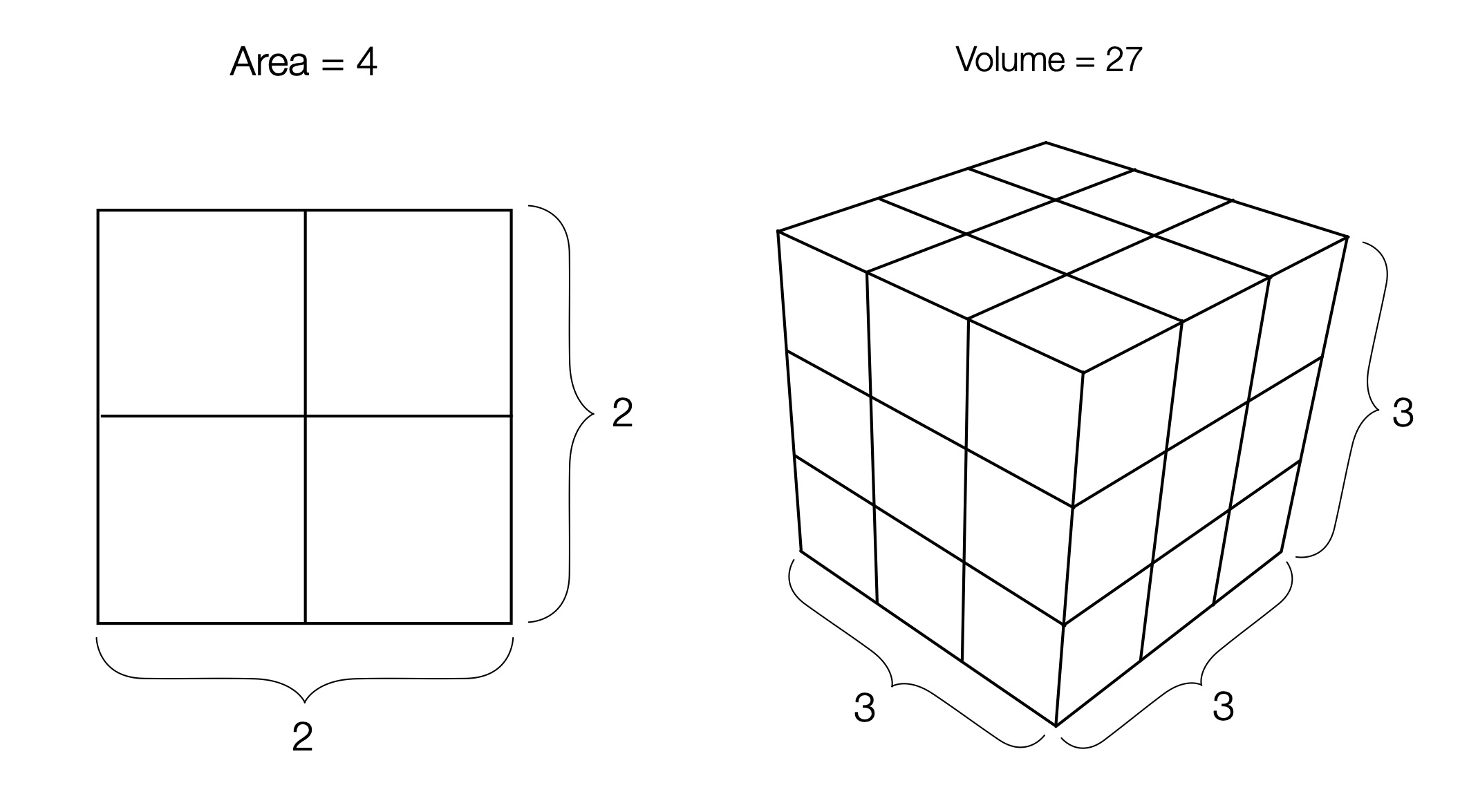
Figure 3: Square / root and cube / root, illustrated.

Roots are the inverse operation of powers. Referring back to the figure you can see that the square root of 4 equals 2; square root is the number that would be “squared” to construct a square of area equal to 4, so the square root is the length of the side. Similarly, the cube root of 27 equals 3; the cube root is the number that would be “cubed” to construct a cube of volume equal to 27, so the cube root is the length of the side. It gets a bit awkward after cube roots (and cubes for that matter) since a geometric construction like that above would have to be drawn in 4-dimensional space, or higher. Don’t worry – I don’t know how to do that either.

Fractional powers can be confounding since they aren’t as intuitive as whole powers. Fortunately, there are a few simple ones that will get you started. For example, the square root can be written equivalently as raising something to the power of one half:

$\sqrt c = c^{\frac{1}{2}}$

and the cube root is the same as raising something to the power of one third:

$\sqrt[3] P = P^{\frac{1}{3}}$

Next, a constant or variable raised to a negative power is the same as dividing 1 by the constant or variable raised to the same power, with the power now positive. This is most easily understood with a couple of examples:

$x^{-2} = \frac{1}{x^{2}}$

$P^{-\frac{1}{3}} = \frac{1}{P^{\frac{1}{3}}} = \frac{1}{\sqrt[3]{P}}$

Finally, fractional powers can be written as products of other powers, generally a whole power and a fractional power. This is useful if you wish to group terms in some meaningful way, such as something squared being indicative of an area. So here are two examples, one quite general (where the fractional power is comprised of two constants) and another that’s more concrete:

$x^{\frac{m}{n}} = x^{m} x^{\frac{1}{n}}$

$L^{\frac{2}{3}} = L^{2} L^{\frac{1}{3}}$

Functions

When I was a high school senior I took a Calculus I class at nearby Colby College since my high school didn’t offer this subject. The greatest conceptual leap I had to make was to embrace functions. Prior to the class I had always done fairly concrete mathematics: add some numbers, factor an equation, solve a quadratic, plot a line, do a geometry proof. There was almost nothing abstract about it, and we seldom looked to generalize our work.

But I learned functions are no big deal, and actually a very useful concept. Think of a function as an input-output black box as suggested in Fig. 4. You give it an input, and an output emerges. “Function” is just another way of saying “one or more mathematical operations performed in a prescribed way upon one or more constants, variables, or functions.” The last part about functions performing operations on functions is a bit abstract – just hold tight.

The operations that comprise a function may include combinations of familiar arithmetic operations like addition, subtraction, multiplication, and division, as well as powers and roots. Trigonometric functions like sine and cosine, which themselves are functions (give ‘em an input angle and they return an output result), can be used in constructing a larger, more complex function.

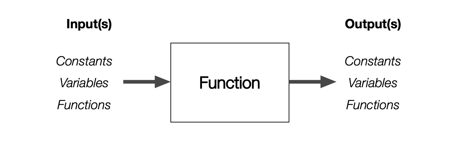
Figure 4: A function as an input-output black box.

A function that operates on a single variable x can be written using shorthand such as f(x), pronounced “f of x.” ‘f’ is the function. Any other letter or symbol could be used to designate it; f is just a convenient choice and nothing more. The input variable x, often referred to as the function’s argument, is called an independent variable since the function depends upon it and not the other way around. If the output of the function is another variable, say y, then y is called a dependent variable since it depends upon the function f as well as the independent variable x.

This can all be expressed succinctly, and rather abstractly, as

$y = f(x)$

Note that we haven’t specified what the function f is or what it does. This is by design; it was here that I was tripped up so often when first introduced to this nomenclature. But the power of this very general form of representation lets us define f as, for example,

$f(x) = \frac{1}{2} \rho A C_{D0} \cos x$

$f(x) = m \frac{dv}{dx} + C_{1} v + C_{2} v^{2}$

and thereafter never have to write down all these operations again since the interested reader can refer back to the details as required. It is merely a convenience, a shorthand, like naming the thing you are sitting on “chair” without the need for naming and listing each and every one of it component parts, the materials from which it is constructed, dimensions, color(s), upholstery fabric and pattern, etc., every time you refer to it. It’s more compact, too.

A function can be as simple as one arithmetic operation, like addition. Or we could define a function – we’ll call it the “Douglas Adams” function^[4] – that multiples an input variable x by 42:

$f(x) = 42x$

This means you’ve been using functions ever since you started doing multiplication tables. Surprise! Granted, this function isn’t very interesting. But it provides another straightforward example in reading mathematics. If x goes to zero in our Douglas Adams function f we see that f goes to zero as well. If x becomes very large f also becomes large; 42 times as large as a matter of fact. If x is negative f is also negative. This is how you actively read a function: look for where it equals zero, what happens if its input variable(s) go to zero or become large, how it behaves with positive and negative inputs.

Consider now the function

$f(C) = 1.8 C +32$

If C = 0 then f goes to 32; if C = 100, f becomes 212; if C = -17.8 then f goes to (approximately) 0. We have defined a function f that converts from degrees Celsius to degrees Fahrenheit. As you can see functions are no big deal, and nothing to get wound around the axle about.

Things get more interesting with

$f(x) = \frac{x^{2}}{(1-x)^{3}}$

When x = 0 this function also equals zero – try it and see. What happens when the independent variable x gets large? By “large” we mean that x assumes a magnitude, positive or negative, large enough that the 1 in the equation’s denominator can be ignored in comparison. In that case the function f is approximated by

$f(x) \approx \frac{x^{2}}{(-x)^{3}} = \frac{-1}{x}$

As x gets larger and larger in magnitude f will become smaller and smaller, eventually approaching zero. The negative one in the numerator indicates that the value of f will be negative for large positive values of x, and positive for large negative values of x – remember, this is an approximation that is only valid for values of x with magnitude much larger than 1. And finally, something interesting happens when x = 1. The numerator then equals 1; great. The denominator, however, will equal 0. Dividing anything finite by 0 equals infinity, therefore f becomes infinite at x = 1. Who knew there were so many things going on in this apparently simple equation? You do, because you are reading mathematics.

There are a few common trigonometric functions worth knowing about like sine and cosine, along with the transcendental functions^[5] of exponentiation and logarithms (trig functions are also transcendental functions; there’s your extra credit for the day). We’ll save those for the next section on plots. There are also two key functional operators from calculus: derivatives and integrals. We’ll visit with them later on as well.

Plots

Plots are visual representations of the mathematical relationship between variables and/or functions. They are also a means for visual learners to read mathematics, complementing what we learned about reading functions above. An example appears in Fig. 5.

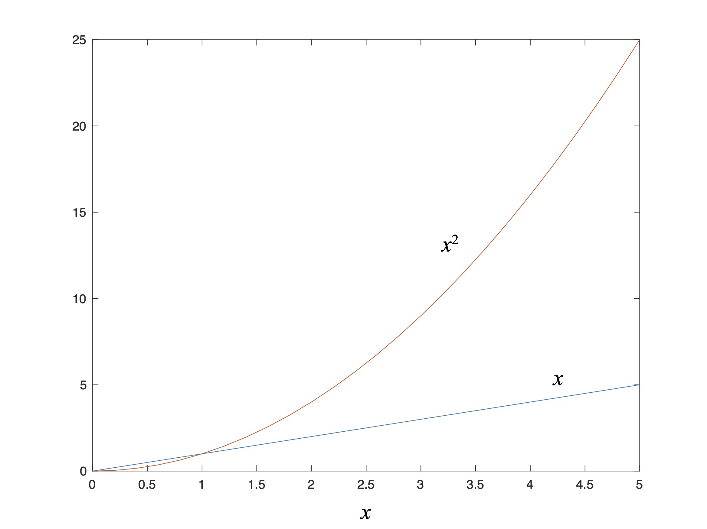
Figure 5: Plots of x and x² vs. x.

This plot compares x and x² over a range of values of x. While it doesn’t look like much this plot illustrates a few helpful tips for reading mathematics. First, notice what happens when x = 1: both curves intersect.^[6] Between 0 and 1 the magnitude of the square of x is smaller than x, something that is always true for numbers between 0 and 1 for any power of x – higher powers of x are always smaller in magnitude than lower powers of x when x is between 0 and 1. And above this the magnitude of the square of x is greater than x; this is true for all powers of x – higher powers of x are always larger than the lower power when x is greater than 1. These two “small” observations come in handy over and over again in applied mathematics when we are looking at limiting cases – e.g., when is one change larger / more significant than another – or to simplify the math by dropping terms that are much smaller than other. Master these straight-forward observations and you will go far.

But where do plots come from? The 2D plot in Fig. 5 above is a way of representing the relationship between numbers in a Cartesian^[7] coordinate system. These numbers often correspond to physical quantities like space or time, force or power. In that way Fig. 5 is a little bit like a map, with two coordinate axes – here, values of the independent variable x (with horizontal coordinate axis called the abscissa) and the values of two functions of x (with vertical coordinate axis called the ordinate), rather than latitude and longitude.

When I first learned how to plot functions I went through the process of drawing a Cartesian grid, creating a table with ordered pairs of values for x and its function(s), then placing a dot on the grid for each pair. Nowadays I use Matlab or Excel to generate these plots, or because I’ve plotted many functions over the years I can draw a good approximation in my notebook to at least get started.

When reading any plot first look at the ranges of the abscissa and the ordinate, as well as what the labels tell you is being represented. Is this a plot of how something varies over time? Over space? With respect to a variable parameter? This gives you the lay of the land. Then, how many relationships (in the form of plotted curves) are there? If there is more than one curve, what does each represent, and how do the curves relate or differ? Is something getting small, or large, or changing from positive to negative for one or more values or ranges of the independent variable or variable parameter? Here you’re looking for trends since the plot represents the relationship between variables and functions in a visually accessible way; this is their great value. In short, you’re asking the plot, “What are you telling me?”

Consider now the plots of x and its square and cube roots in Fig. 6.

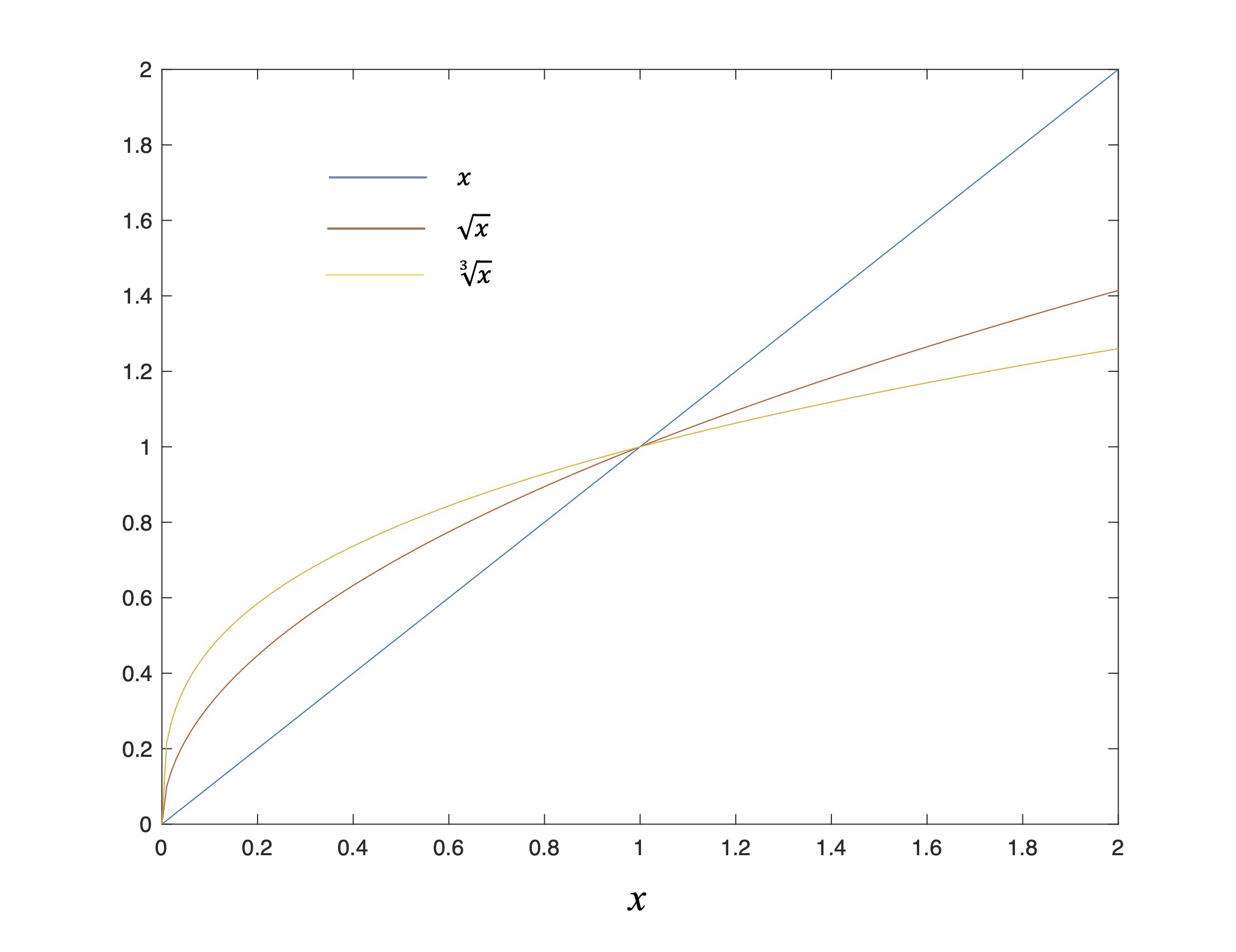
Fig. 6: Plot of x along with its square and cube roots vs x.

Figure 6, like Fig. 5, shows the relationship between x and two of the powers of x except that now these powers are fractional: the $\frac{1}{2}$ power (i.e., the square root) and the $\frac{1}{3}$ power (i.e., the cube root). Like before, something interesting happens with these three functions around x = 1. Using your ability to read mathematics, what can you say about larger vs. smaller fractional powers on either side of x = 1?

One last twist to plotting is that sometimes you’ll find that the horizontal and/or vertical axis scales are… weird. Not evenly spaced. If either the independent variable or corresponding functional values extend over a wide numeric range it sometimes makes sense to use a logarithmic spacing along one of the plot axes.

Logarithmic spacing isn’t all that unfamiliar since that’s how your hearing perceives sound, both in how you can pick out its various tones as well as how you perceive changes in the volume of sound. For instance, the keys on a piano are assigned to notes such that every octave, or doubling of sound frequency, corresponds to twelve keys (the white ones and the black ones combined). Successive doublings like this is an example of logarithmic (aka, “log”) spacing. Who knew you already were familiar with log spacing? Then, if you’ve ever read of a sound level expressed in decibels (aka, “dB”, a unit of measure named after Alexander Graham Bell, inventor of the telephone), well, those are logarithmic values of sound amplitude since our ears can more easily distinguish successive doublings of sound amplitude. Our range of hearing covers 120 dB of amplitude from softest to loudest, or a range of 1,000,000,000,000 (one trillion). If you had to plot numbers on a linear scale of zero to one trillion the graph would be awfully large.

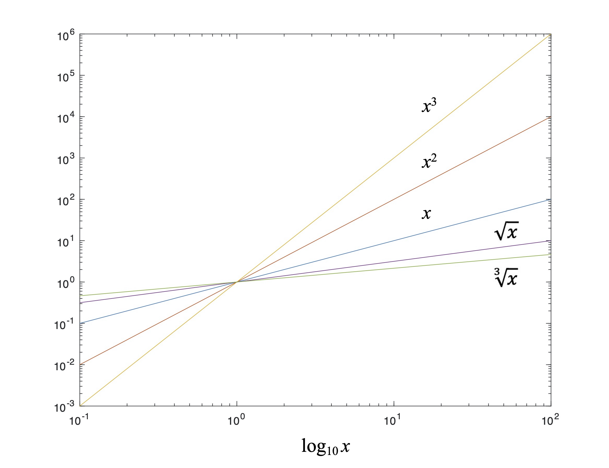
Figure 7: Logarithmic plot of various powers of x.

Fig. 7 is an example of a plot with log axes where we revisit a few old friends: powers of an independent variable x. Since we (now) know that taking the root of a variable is the same as raising it to a fractional power this plot tells us something interesting. When plotted on log axes any power of a variable is simply a straight line. This doesn’t mean that powers of a variable are straight lines (!), only that their plots on logarithmic axes are. The various slopes of the straight lines in Fig. 7 simply represent the power of x, aka its exponent. Fig. 7 embodies the following mathematical identity:^[8]

$\log x^{n} = n \log x$

This identity, like our logarithmic plot, shows that the log of anything raised to a power (whole or fractional) is the same as the power times the log of said thing. For those of you who grew up using “slope and y-intercept” rules for plotting straight lines, all Fig. 7 does is use log x as the independent variable, and the exponent as the slope. It was this insight into the logarithm of powers that enabled me to write Part 12: The Deflection Point.

Now that we have the basics of plotting under out belt we can use this tool to provide visual summaries of a few common trigonometric and other transcendental functions. First, Fig. 8 is a plot of the sine and cosine functions:

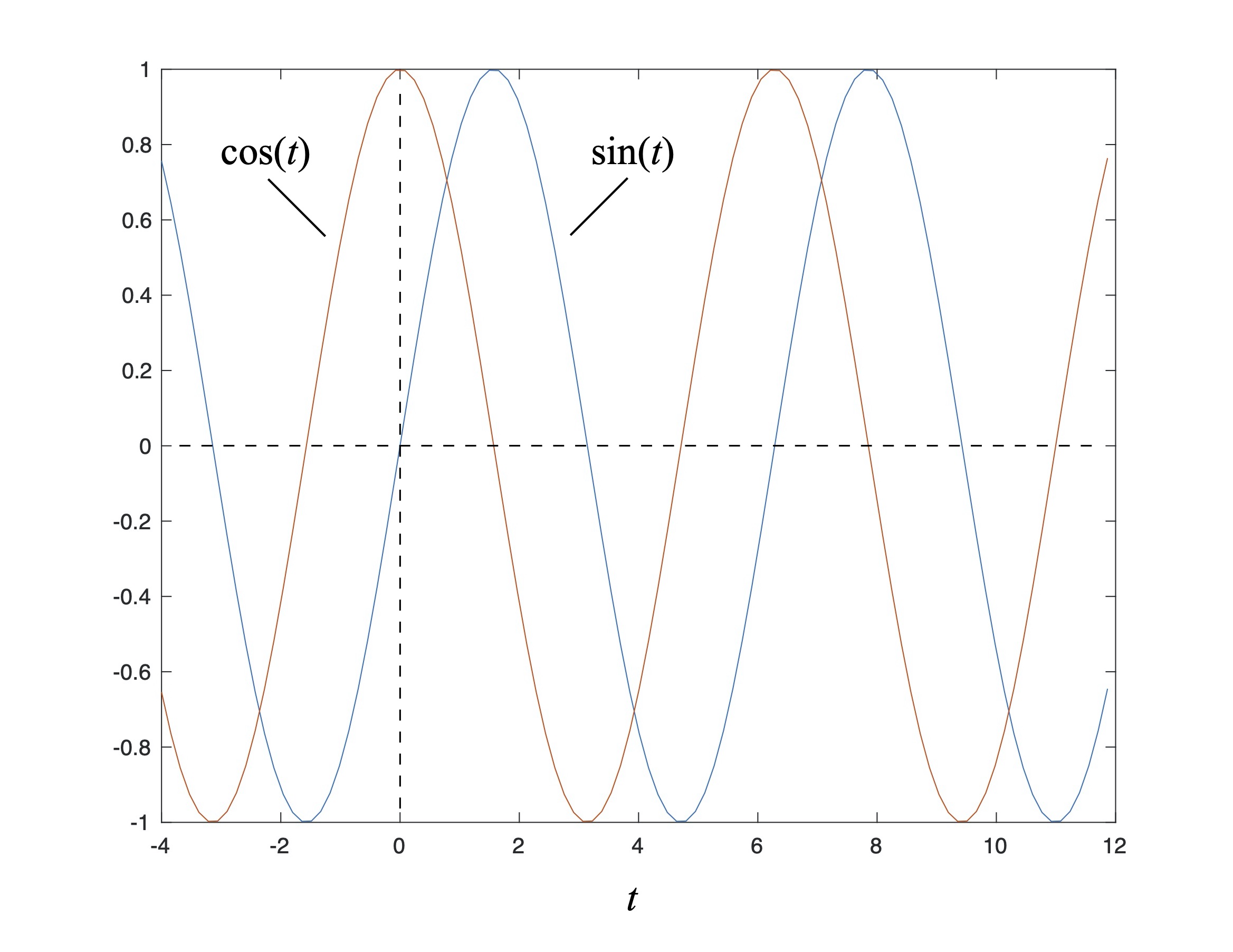
Figure 8: Plot of sine and cosine.

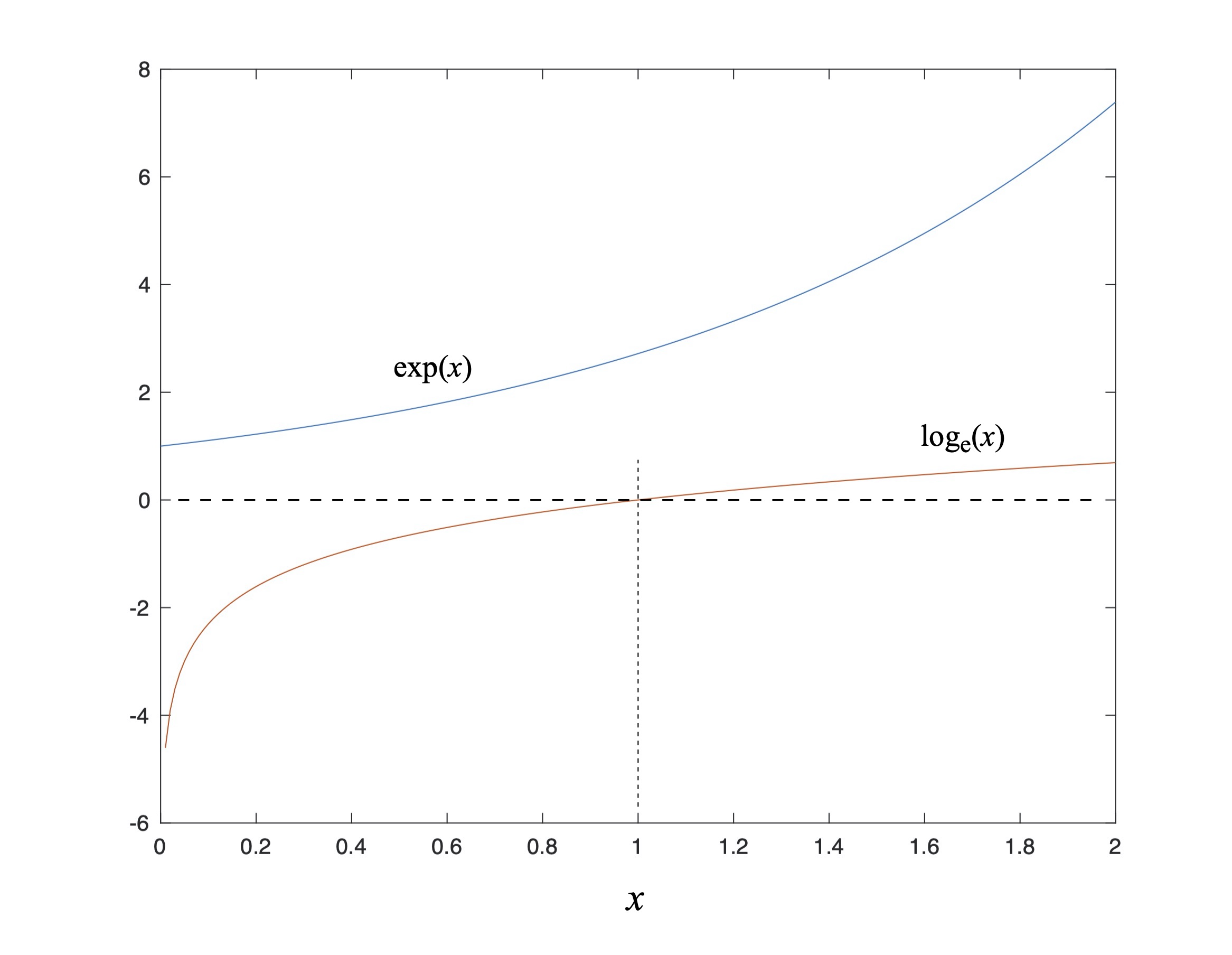
Note how the periodic sine and cosine functions are identical to each other except that they are shifted along the t axis of the plot by $\pi$ /2. Their amplitudes always and only vary between -1 and +1. And the sine function is zero when its argument t is zero, while cosine is 1 there; this pattern repeats itself along the horizontal axis in 2 $\pi$ increments. If the horizontal axis represents time then the spacing that corresponds to this repetition is called the period; if the horizontal axis represents space then this repetition distance is called the wavelength.

Figure 9: Plots of exponential and natural log.

Fig. 9 is a plot of the exponential and natural logarithm functions – note that exp(x) is sometimes written as e^x. Aside from noting where each function grows or decreases in magnitude, and where one becomes negative, you can also see that the natural logarithm (i.e., the logarithm in base e – more on that in a moment) of 1 equals 0, while the exponential of 0 equals 1.^[9] This curious symmetry arises in part from the relationship between the exponential and the natural logarithm: they are inverse functions of each other. In other word the natural logarithm of the exponential of an independent variable returns the independent variable: the function of its inverse function returns the argument, and this is one example. You can see this very simply (for once!) via the equation

$\log_{e}(e^{x}) = x$

The exponential function is just raising the number e to the power of x, and we (now) know that taking the log of anything raised to a power is equal to that power times the log of said thing. Which means that

$\log_{e}(e) = 1$

So the natural logarithm function is defined in a backwards fashion based on its properties: it is the inverse function of the exponential (hence the “base e”), and the logarithm of powers does that nifty linearization thing. Remember Mrs. Hazen’s advice, and don’t worry about what logarithms are, but what they do; in other words, don’t overthink it.

[For extra credit, where did this constant e come from? ‘e’ is called Euler’s Number in honor of the Swiss mathematician Leonard Euler – even though he didn’t discover it. It is the basis of Euler’s Identity, one of the more remarkable statements in all of mathematics:

$e^{i \pi} = -1$

an identity that includes the transcendental numbers e and $\pi$ , the transcendental function of exponentiation, the imaginary number i (which is the square root of -1), as well the negative number, -1. But e itself was discovered by Jacob Bernoulli^[10] while exploring the mathematics of compound interest, something a bit more mundane but far less abstract.]

Lastly, plots are an easy way to visualize whether a function has even or odd symmetry. Even functions return positive results for all values – positive or negative – of its independent variable, while odd functions return positive results for positive inputs, and negative values for negative inputs. For example, Fig. 10 shows that odd powers of x have odd symmetry about x = 0, while even powers of x have even symmetry about x = 0. Along the same lines Fig. 8 shows that the sine function has odd symmetry about 0, while cosine has even symmetry.

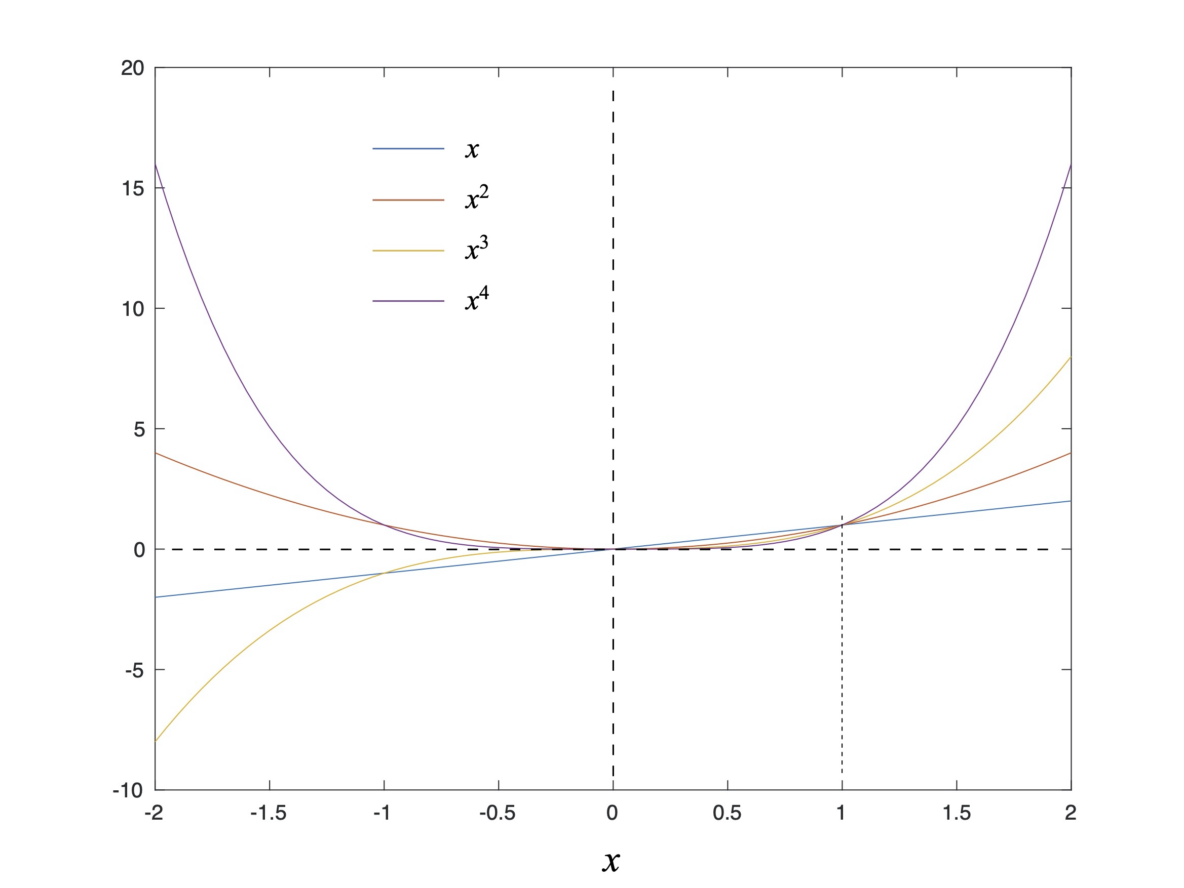
Figure 10: Powers of x showing their odd and even symmetries.

Why do we care about even and odd functions? It is often useful to understand when or if a function flips sign from positive to negative – if the function represents a physical process this may indicate (for example) a change of direction, acceleration versus deceleration, or a change in direction of power flow from source to sink. Next, the product of any two even functions is also even. The product of any two odd functions is even, while the product of an even and an odd function is odd. Factoring a function into a product of even- and odd-symmetric parts, each of which might correspond to a physical process, can lend insight into the underlying processes and their interrelation. Understanding even- and odd-symmetric functions made my doctoral thesis possible, leading to a series of publications and patents by myself and others, along with devices that up until then had never been built let alone conceived of. Go figure.

As you have… seen… plots make a number of mathematical concepts more accessible and concrete. Use them liberally and wisely.

Derivatives

Ordinary derivatives^[11] are operators that represent the rate of change of some function with respect to an independent variable; you would say or write that the derivative is with respect to that variable, as in the “derivative with respect to time” or the “derivative with respect to x.” In Science of Paddling articles we are concerned with quantities that vary over time, such as position and force, as well as over space, such as the velocity across a wake. But for the most part we work with derivatives where time is the independent variable and so you’ll mostly encounter time derivatives. While derivatives are typically one’s first entry point into calculus we won’t be asking you to do them (unless you want to), only read them. It’s not hard.

A few of the most common derivative expressions you’ll encounter in TSOP are those that define the relationship between position x, speed v, and acceleration a:

$v = \frac{dx}{dt}$

$a = \frac{dv}{dt} = \frac{d^{2} x}{d t^{2}}$

What looks like fractions above are actually derivatives; the notation comes from Gottfried Leibniz, who developed calculus at around the same times as Isaac Newton but beat him to publication.^[12] What looks like squared quantities actually indicate taking a second derivative: acceleration is the derivative with respect to time of velocity, which itself is the derivative with respect to time of position, hence acceleration is the derivative of the derivative of position or the “second” derivative of position with respect to time. Also note that the time dependence of position, velocity, and acceleration is implicit in the above expressions; this saves writing, for example, velocity as v(t). Lastly, you may sometimes encounter the term “differentiation,’ which means to take the derivative of some function; it’s just terminology. And that’s really all you need to know; skip to the next section if you wish.

What follows in the balance of this section is a sidebar for those who want a more intuitive understanding of the derivative operator. First, note that the ‘d’ in the derivative notation suggests an infinitesimal change in the variable adjacent to it. The dx represents an infinitesimal change in position x, while dt represents an infinitesimal change in time t.^[13] And what is an “infinitesimal”? A quantity that is smaller than any number, but not equal to 0. This definition gives rise to the phrase “arbitrarily small.” Great; arbitrarily small. How does this relate to derivatives representing a rate of change?

It’s pretty easy to explain using a plot. Consider the arbitrary continuous^[14] function f(x) plotted in Fig. 11. Looking at the plot, where do you see this function changing more or less rapidly with respect to x? Certainly, at x = a the function is changing more rapidly than at x = c; small changes in the independent variable x around x = a lead to greater changes in f(x) than around x = c. How are we able to infer this? By the slope of the function f(x) around those locations. The slope of a function at a point reflects its local rate of change: no slope, no change; lots of slope, lots of change. So if f(x) represents the position of your hull over time, and x represents time, then a steep slope in some portion of the position versus time plot means you’re moving fast, a gradual slope means you’re moving slowly, and a flat slope means that your position over time isn’t changing and you’re stationary.

Figure 11: A continuous function.

Now about those infinitesimals. Consider the right triangle shown in Fig. 11 with two of its vertices intersecting the function at x = a and x = b. The triangle’s hypotenuse connects these two intersection points; the hypotenuse is thus coincident with the secant to f(x) there. The side labeled ‘d’ is the width of the triangle, while ‘h’ is its height. The ratio of this triangle’s height to its width corresponds to the slope of the hypotenuse (and the secant mentioned above); I recall learning this as the ratio of “rise over run.” We can define the slope of this hypotenuse via values of the function at the locations x = a and x = b (which equals a + d) and the width d:

$slope = \frac{f(a + d) - f(a)}{d}$

This fraction has a numerator that can be read as the incremental change in a function (such as position), and a denominator that can be read as the incremental change in its independent variable (such as time); sounds like the way we interpreted Leibniz’ derivative notation, eh?^[15] As the triangle’s width d gets smaller and smaller – as it becomes infinitesimal – the secant approaches the tangent to f(x) at x = a. This tangent is the slope of the function at that point, and thus is by definition is the derivative of the function there. So to define the derivative of the function at x = a we plug in the form of the function f and let d go to zero. To derive the derivative of this function everywhere we can go through this process for each and value of its input. Or, we learn the derivatives of a few common functions, look up the derivative in a book or online, or both!

Summations

Summations are just a compact way of representing a sum of many parts. Here’s an example:

$total = \sum_{i=1}^{N} s_{i}$

“Total” is, well, the total of the sum. The large sigma (“S”) indicates that whatever sits to its right are the things being summed: the summand. In the example above there are a number of quantities represented by the symbol s to be added together. The subscript ‘i’ in an index for the things being summed. The subscript beneath the sigma indicates that we’ll start the summation with the first index i = 1, which corresponds (we assume) to the first item s_i; note that the sequence can start at an index other than 1, and the sum may sometimes only be over a subset of the items s_i, so read the summation carefully. The superscript above the sigma indicates that the last item here will have index N, where N is some constant. In many cases a specific number appears here.

The summation above is saying, “add together N items ranging from the first to the N^th.” That’s it; summations are just a convenient and compact way of writing

$total = s_{1} + s_{2} + s_{3} + s_{4} + s_{5} + ... + s_{N}$

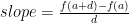
One example of summation’s utility is in approximating the area under a curve. Let’s say that someone owns a lot along a lakeshore where the shoreline has a shaped described by the curve in Fig. 12, and their lot is bounded on the West by x = 1, and on the East by x = 5. (I know; work with me here.) They want to know the size of the lot in order to not overpay their property taxes.

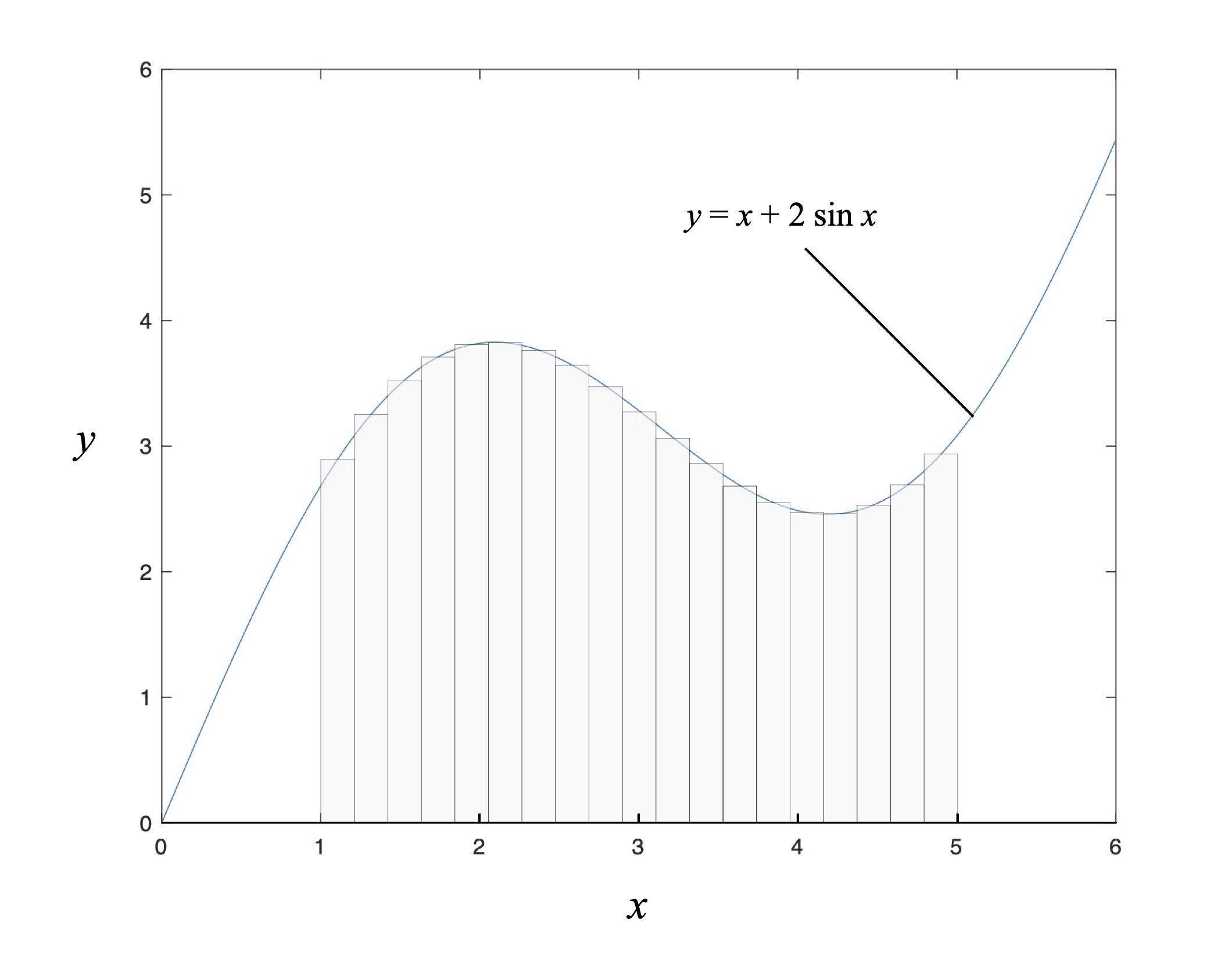
Figure 12: Approximating the area under a curve.

Since this shoreline has a wonderfully regular shape described by the function x + 2 sin x (I know; work with me) they can divide their lot into a series of plank-shaped rectangles having uniform width d, compute the value of the shoreline shape function at the midpoint of each rectangle to get the corresponding rectangle’s height, then multiply these two quantities to calculate the area of each rectangle. Sum these all up and voila! An approximate acreage of their plot.

If there are N rectangles, and each rectangle has area A_i, then the acreage is approximately

$Acreage \approx \sum_{i=1}^{N} A_{i}$

For extra credit… if we denote the value of the shoreline shape function at the center of each rectangular area by f_i, then each area is

$A_{i} = d \times f_{i}$

where the width d is a constant.^[16] Then our summation for the acreage can be written as

$Acreage \approx \sum_{i=1}^{N} d \times f_{i} = d \sum_{i=1}^{N} f_{i}$

where we have taken d outside of the summation since it is constant – this is just the distributive property of multiplication in action.

Now consider this last summation in light of Fig. 12. Intuitively, we can see that by using narrower and narrower rectangles to approximate the area under the shoreline curve our acreage estimate will be more accurate – we’ll just have to use more terms in our summation, e.g., N will become larger, and d will consequently become smaller. So if we imagine the width d becoming infinitesimally small until it approaches zero, and consequently N becoming larger and larger until it approaches infinity, we either end up with Zeno’s paradox^[17] or… integrals.

Integrals

Definite integrals assign a value to a function over a finite interval of its independent variable by adding together – i.e., integrating – an infinite number of infinitesimal areas. This is illustrated in Fig. 13 for the function x + 2sin x over the interval from 1 to 5, where the shaded region represents the area. This is the continuous version of the acreage problem illustrated in Fig. 12; definite integrals and sums are related.

Figure 13: Area under a curve.

This integral is represented mathematically by

$\int_{1}^{5} (x + 2 \sin x) dx$

The integral sign is the stretched italic ‘S’ – when you see one of these it means integration. The subscript ‘1’ is the starting point for the operation, also referred as the lower limit of integration; the superscript ‘5’ is the end point of the operation, also referred to as the upper limit of integration. Everything to the right of the integral sign aside from the dx is the integrand, or the thing to be integrated (like the summand were the things to be summed). ‘dx’ is a differential of the independent variable x, indicating that integration is to be performed with respect to this variable as opposed to something else. It also echoes the role of the definite integral in computing the area under the curve defined by the integrand since dx is infinitesimal. Definite integrals do in fact compute areas; that’s the most straightforward way to think of them.

More generally, the definite integral of a function of one variable f(x) can be written as

$\int_{a}^{b} f(x) dx$

where a and b are the limits of integration, and x is the independent variable. Whenever you see an integral written with limits like this the result will be a constant since the integral “integrates away” the independent variable. The result might be expressed in terms of other constants, like the density of water or its kinematic viscosity, but the independent variable will no longer appear after taking the integral. The result will be some amount, such as… an area.

Now the thing about functions is that they can have positive or negative values over certain ranges of their arguments. Consider the function depicted in Fig. 14: 2 – x + sin(3x). Between 0 and 2.5 it takes on both positive and negative values. As a result, the definite integral of this function over the interval from 0 to 2.5 will be comprised of two areas with a positive value and one “negative” area. We tend to think of the “area” of something as a number that is greater than zero; who ever heard of negative acreage?

But integration is more literal than intuitive. Which means there can be negative areas as well as positive ones. For example, if the line y = 0 in Fig. 13 described the original shape of a sandy shoreline (again, work with me here), and the function 2 – x + sin(3x) describes a desired new shoreline shape that would be built up using sand, then the integral tells you how much sand to buy for building the new shoreline in light of how much you could reuse by excavating the “negative area” portion. This somewhat superficial example underlies an important fact: definite integrals can return a value of zero, and when they do usually something important and worth your attention is going on.

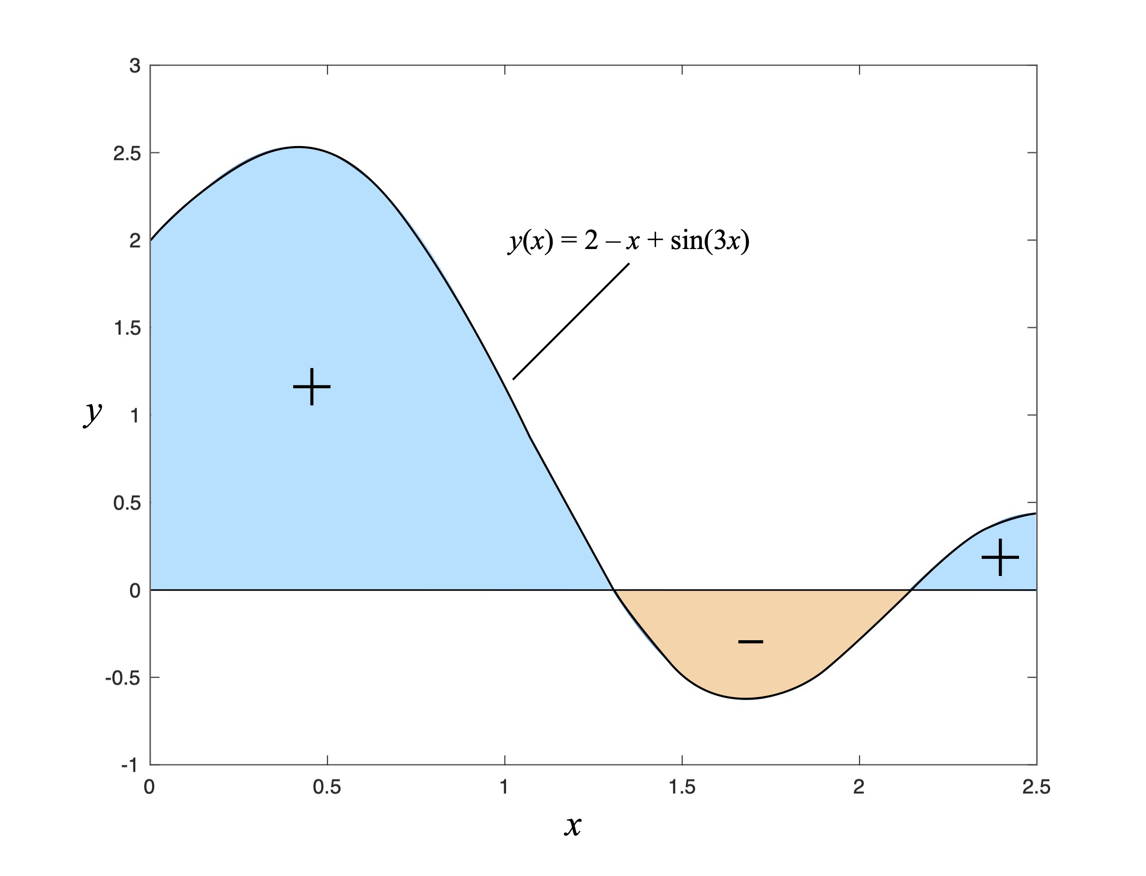
Figure 14: Integration of a function having positive and negative areas under the curve.

You can perform integration over multiple dimensions if the integrand depends on more than one independent variable. For example, the flow velocity across a hull’s wake varies over both the wake’s width as well as its depth; to compute the force from the flow’s dynamic pressure due to the wake you need to integrate over the wake’s cross-sectional area – see Part 26: Waking Up for an example. The result is still a constant; remember, definite integrals “integrate away” independent variables.

You might now be wondering what all the fuss is regarding the terminology “definite integral” rather than just “integral.” It’s because there is also a type of integral called an indefinite integral; you can spot them by the fact that they have no limits of integration, such as

$h(x) = \int f(x) dx$

Notice that indefinite integrals are written (sometimes implicitly) with a function on the left-hand side of the integral sign. This is because they don’t “integrate away” the independent variable, but instead return another function.

For extra credit: the functions h and f – whatever they may be in order to satisfy this mathematical statement – have a unique relationship: h is the integral of f, while f is… wait for it… the derivative of h. This last sentence requires a few qualifications that aren’t important here. But a nifty piece of mathematics called the Fundamental Theorem of Calculus proves that integration and differentiation are inverse operations; two sides of a coin. This is why you can move from position to velocity to acceleration via differentiation, and from acceleration to velocity to position via integration. Useful stuff.

Equations

Equations are just various combinations of the things described above, where one thing is set equal to another (hence, “equation”). That’s it; you’re done. Here’s an example:

$F=\frac{1}{2}\rho A{{C}_{D0}}\cos \left( \theta -\phi \right)\left( {{v}_{hull}}-{{v}_{paddle}} \right)^{2}$

So how do you put all this together to read an equation? Here are some guidelines:

Take your time.
In case you forgot, take your time!
Look at both sides of the equals sign. What is being equated with what?
Then look at the groupings of terms – the clumps of constants, variables, operators, etc. For each, what does it mean in plain language? For example, is one grouping an integral, and if so what does it represent? Force; impulse; something else? In this step you’re just scanning the equation for its overall structure in order to determine what concept(s) is(are) being conveyed.
The equation may contain a number of constants. In a well-written paper or text these will be defined by the author. Certain constants like $\pi$ , g (the acceleration due to gravity), or e are well known in various fields, and the author may assume you are part of the in-crowd who is familiar with them.
Next, identify the variables and determine what they are and where they are used. The equation will define the relation between these variables.
Does one side of the equation equal zero? If so, can you determine what causes everything on the other side of the equation to equal zero? If the populated (non-zero) side is comprised of two more things added (or subtracted) together this means some things have to cancel each other out to equal zero. What does each part of this summation mean, and what does it mean if they cancel each other?
Does a variable appear by itself on one side of the equals sign? If so, that variable may be an output (like a force, a velocity, or the like) or something else of particular interest, an unknown quantity defined by the rest of the equation.
Try to visualize how changing one variable effects the output / unknown quantity, or look to see limiting cases like when one variable gets large or small compared to another (or large / small in an absolute sense), or what might cause the numerator or denominator of a fraction to go to zero, or what might cause the argument of a function to go to zero, or what happens when a variable goes to zero. Keep in mind what range of values the variable(s) and any parameter(s) can take on in order for your inferences or conclusions to be consistent with physical reality.

So let’s go back to the equation from the beginning of this section, and read it.

$F=\frac{1}{2}\rho A{{C}_{D0}}\cos \left( \theta -\phi \right)\left( {{v}_{hull}}-{{v}_{paddle}} \right)^{2}$

The author has defined F as the paddle blade force, A as the blade area, C_D₀ as the blade’s drag coefficient, $\theta$ as the shaft angle with respect to the vertical, $\phi$ as the bend angle of the blade with respect to the shaft, and v_hull and v_paddle as the forward velocities of the hull and blade, respectively. You understand that in the context of this equation $\rho$ is the density of water, both from past experience and the fact that this has something to do with paddling.

The blade force F stands by itself on the left-hand side of the equation. This means it is an output, or the result of things on the other side of the equation happening. Since we know that the hull and paddle velocities vary over time, as well as the shaft angle, we infer that the blade force will also be a function of time.

The fraction and the water density are fixed constants. Nothing more to see there.

The equation shows that the blade force varies in direct proportion to the blade area if every other term in the equation stays the same. Don’t forget this qualifier since it will prove helpful in a moment. You could infer that this relationship means if you want infinite paddling force – and who doesn’t? – you just need a really gargantuan blade. This is where a quote from one of my favorite technical papers comes in: “We need to salt our analyses with liberal doses of common sense.” Even a fairly large blade might not work for someone who can’t pull the blade through the water fast enough to achieve the relative velocity between hull and paddle in the equation, which we assumed would remain the same when parametrically looking at the impact of blade area by itself. So blade force does depend on paddle size; just be careful about running with this fact in isolation from everything else.

The paddle force also varies in direct proportion to the blade’s drag coefficient. The drag coefficient is a function of the blade geometry and associated hydrodynamics. How to alter the blade’s shape to productively effect the drag coefficient is a research project in itself. So for the present let’s assume that it too is a constant.

When the difference between the paddle and hull velocities is zero the paddle force is zero. Check. This may seem like a trivial limiting case. But it’s one of the first things I look for: if the predicted blade force is non-zero when the paddle is not moving with respect to the hull the equation is likely incorrect, and it’s time to go back to the drawing board. Liberal doses of common sense indeed. Further, since the relative velocity is squared this part of the equation is either equal to or greater than 0.

We know from Fig. 8 that the cosine function has a maximum value of 1, corresponding to when its argument equals zero. For the moment we’ll assume that the blade bend angle $\phi$ is zero. This means that the cosine’s argument equals zero when the shaft angle $\theta$ is zero, e.g., when the shaft is vertical (and the blade as well, since we’ve assumed that the bend angle is zero for this now “straight shaft” paddle). If we introduce a bend angle then the difference between the shaft angle and the bend angle must be zero to maximize the cosine, which means for the bent shaft case the argument is zero when the blade face is vertical.

We know from experience that the shaft angle $\theta$ varies with time. This informs our interpretation of the difference between the hull and paddle horizontal velocities, since we know from experience that these variables also depend on time. Given that the fraction, water density, blade area, and drag coefficient are all fixed for a given paddle – e.g., are constants for a that paddle once built – it is the product of the blade angle cosine and this velocity difference that causes the paddle force to vary over time.

So what maximizes the paddle force? This occurs when the cosine of the angle difference goes to 1, its maximum value (e.g., the blade face is vertical), at the same time that the difference between the hull and paddle horizontal velocities is maximum. This interpretation echoes what rowers are told to do: after loading the blade and starting to pull, focus on hand speed to maximize blade force. Turns out the same advice holds for paddlers. And we read it all in an equation.

v. 1.0

No, not that Bernoulli. ↑
Named after German physicist Heinrich Hertz, who played a key role in the early development of electromagnetic theory. ↑
Constants can also be vectors; just not in Science of Padding articles. ↑
Any Hitchhiker’s Guide fans out there? ↑
Transcendental functions are functions that cannot be represented using a finite number of algebraic operations like adding, subtracting, multiplying, dividing, or raising to a power; they “transcend” algebra. ↑
Yes, a straight line is a curve – a curve with infinite radius of curvature. ↑
Named after French philosopher and mathematician René Descartes, whose visual way of representing the relationships between numbers bridged the gap between algebra and geometry. ↑
Math identities are truisms that show two things that are always identical. Hence, “identity.” ↑
Note that raising anything to the 0^th power equals 1, but work with me. ↑
No, not that Bernoulli. ↑
There are also partial derivatives, which are derivatives with respect to one variable where the thing being differentiated depends on two or more independent variables. The symbol for a partial derivative is a bit different, but the rest is a matter of housekeeping. ↑
Newton placed dots over variables to denote derivatives, a notation that is still found in many dynamics texts; Lagrange used apostrophes, something you’ll find in applied mathematics texts. ↑
Interestingly, the notion of infinitesimal quantities was considered heretical during the Middle Ages since it ran afoul of Aristotle, who contended that physical reality was continuous and thus not reducible to atoms or infinitesimals. And don’t forget Zeno’s Paradox. You can read about all this and more in Infinitesimal: How a Dangerous Mathematical Theory Changed the World by Amir Alexander. ↑
For those of you keeping score at home, if the function has sudden jumps in amplitude (e.g. is not continuous) the derivative technically doesn’t exist at those discontinuities – yipes! – and you have to invent a whole new set of functions called generalized functions to address this limitation. Which is far beyond the scope of the entire Science of Paddling series. Carry on. ↑
And the mathematical formula here looks like Newton’s “difference quotient” – recall that Newton was a co-inventor of calculus. ↑
It doesn’t have to be constant but doing so makes things simpler. ↑
Zeno couldn’t conceptualize how an infinite number of infinitesimal things added together could yield a finite result. His famous paradox is about motion. The argument proceeds as follows: in order to move from where you are to some destination you first have to move halfway there. From there you have to move halfway from this new location to the destination. And so on, moving closer and closer where each time you reach half of the distance from where you are to the destination. Since you always have to move halfway from where you are to the destination, Zeno took this to mean that you would move halfway an infinite number of times but never reach the destination; you’d always end up halfway to there. Infinitesimals and calculus resolve this paradox. ↑

The Science of Paddling

The intersection of physics, physiology, and paddle sport

Category Archives: Uncategorized

Part 27: Reading Mathematics

Constants

Variables

Parameters

Symbols

Multiplication

Vectors and Scalars

Fractions

Powers and Roots

Functions

Plots

Derivatives

Summations

Integrals

Equations